Packages
dash-annotate-cv
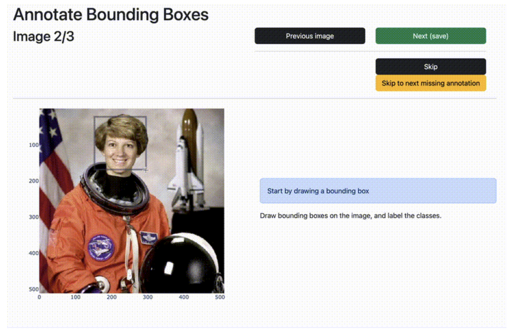
Dash Annotate CV - A dash library for computer vision annotation tasks. dash_annotate_cv is a Python Dash library for computer vision annotation tasks. It exposes reusable annotation components in a library format for dash.
motlinearity
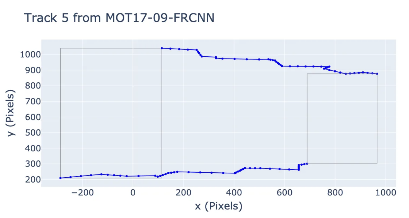
Is MOT piecewise linear? How linearly do people walk? This package provides utilities to analyze the MOT-17 and MOT-20 datasets to find out if people's motions are piecewise linear, and implements some simple methods for detecting piecewise-linear motion, as well as some random walk baselines.
houseofreps
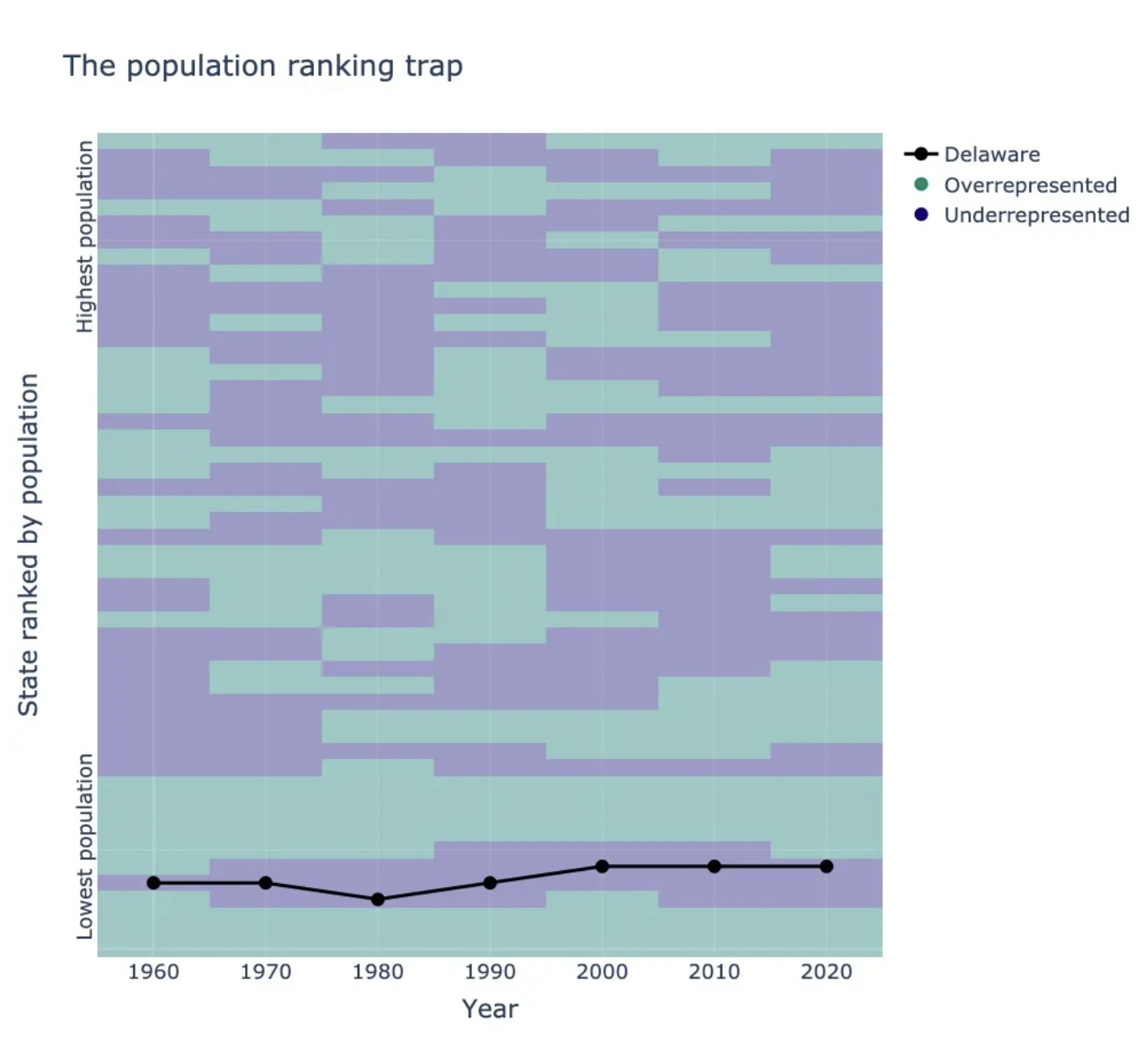
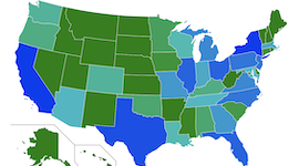
houseofreps implements apportionment methods for assigning seats in the US House of Representatives. Disclaimer - This product uses the Census Bureau Data API but is not endorsed or certified by the Census Bureau. See Terms of Service (https://www.census.gov/data/developers/about/terms-of-service.html).
houseofreps implements apportionment methods for assigning seats in the US House of Representatives. Disclaimer - This product uses the Census Bureau Data API but is not endorsed or certified by the Census Bureau. See Terms of Service (https://www.census.gov/data/developers/about/terms-of-service.html).

physDBD
Python/TensorFlow package for physics-based machine learning. Example applications for modeling reaction-diffusion systems, although the methods are generally applicable.
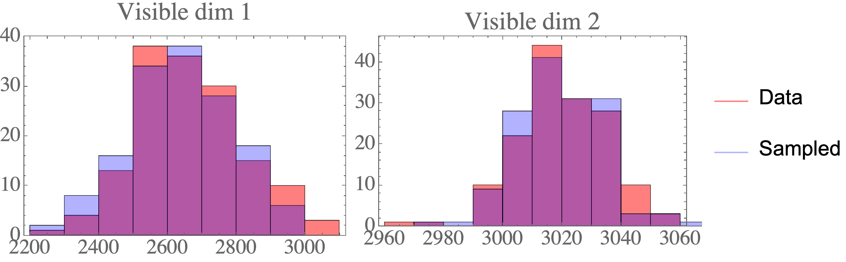
tf-constrained-gauss
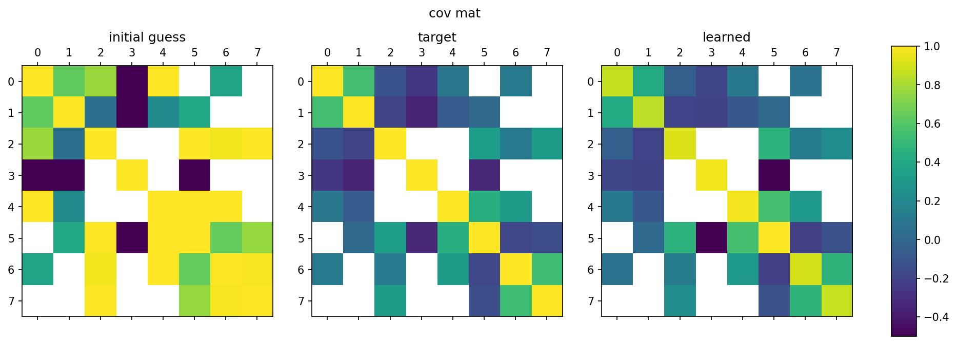
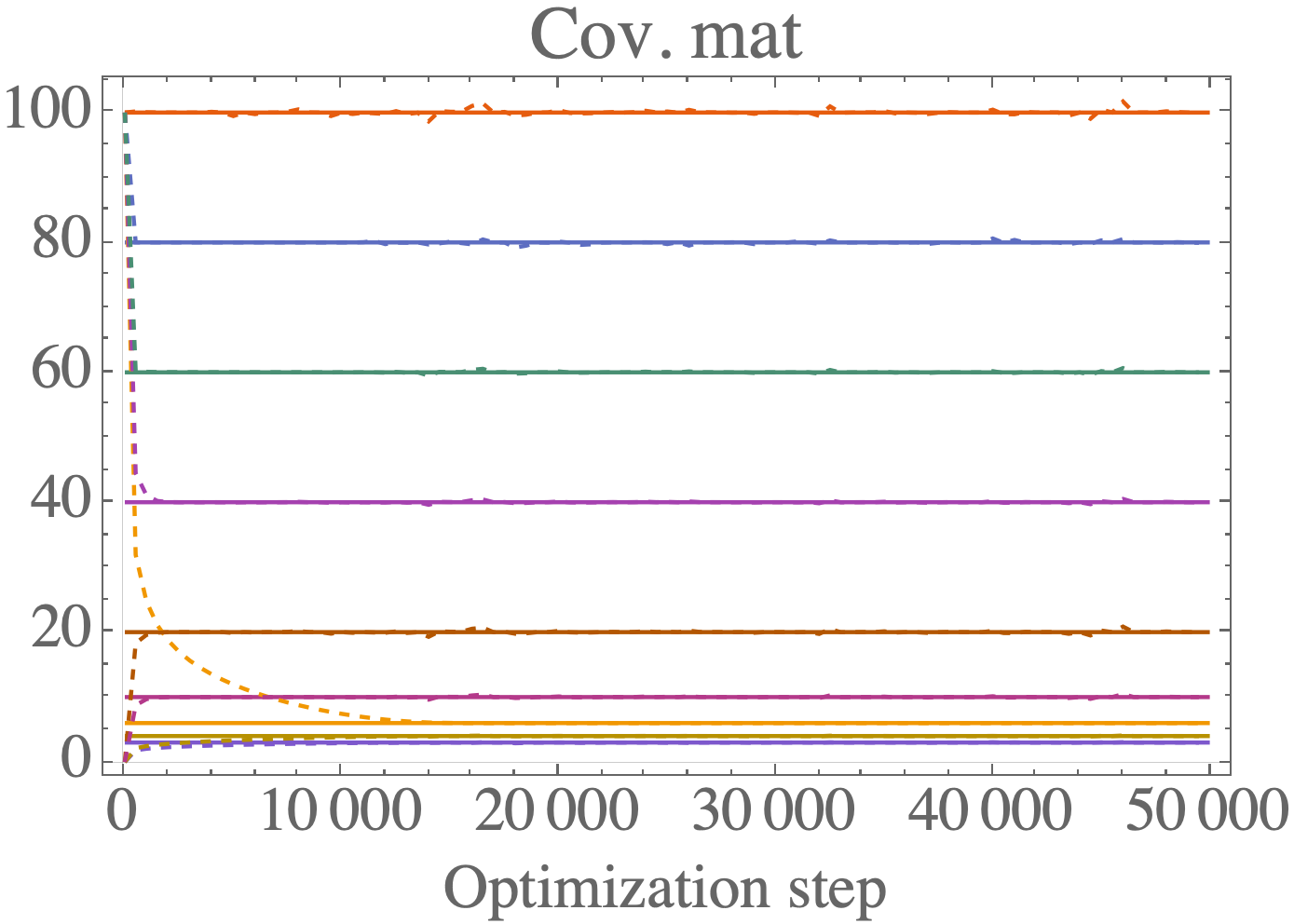
Python/TensorFlow package for estimating constrained precision matrices from mixed constraints. In a Gaussian graphical model, edges between random variables correspond to non-zero entries in the precision matrix. On the other hand, covariances between random variables can be observed from data. This methods implemented are intended to find the precision matrix from (1) the structure of the precision matrix and (2) partial observations of the covariance matrix.
Used in publication: arXiv 2109.05053 (2021)
arXiv: arXiv 2109.05053 (2021)
Python/TensorFlow package for estimating constrained precision matrices from mixed constraints. In a Gaussian graphical model, edges between random variables correspond to non-zero entries in the precision matrix. On the other hand, covariances between random variables can be observed from data. This methods implemented are intended to find the precision matrix from (1) the structure of the precision matrix and (2) partial observations of the covariance matrix.
dblz
A C++ library implementing dynamic Boltzmann machines on a lattice. Includes example applications for lattice chemical kinetics.
ggm_inversion
A C++ library for numerical inversion of constrained precision matrices. The goal of this library is to solve the problem of calculating the inverse of a symmetric positive definite matrix (e.g. a covariance matrix) when the constraints are mixed between the covariance matrix \Sigma and the precision matrix B = \Sigma^{-1}.
A C++ library for numerical inversion of constrained precision matrices. The goal of this library is to solve the problem of calculating the inverse of a symmetric positive definite matrix (e.g. a covariance matrix) when the constraints are mixed between the covariance matrix \Sigma and the precision matrix B = \Sigma^{-1}.
gillespie-cpp
C++ library for Gillespie stochastic simulation algorithm, including tau-leaping. Intended to be used as a stepping stone for your own Gillespie codes.
pairwiseDistances
Python package to calculate and maintain pairwise distances between n particles. A common problem is to calculate pairwise distances for n particles. This occurs in particle simulations (e.g. electrostatics) and many other scientific fields. This module aims to perform this calculation and implements several common efficiency strategies.
Python package to calculate and maintain pairwise distances between n particles. A common problem is to calculate pairwise distances for n particles. This occurs in particle simulations (e.g. electrostatics) and many other scientific fields. This module aims to perform this calculation and implements several common efficiency strategies.
samplePairsGaussian
Python package to sample pairs of particles in n dims from discrete Gaussian distribution. Given a set of n particles with positions in d-dimensional space denoted by x_i for i=0,1,...,n. We want to sample a pair of particles i,j where i =/= j, where the probability for sampling this pair is given by p(i,j) ~ exp( - |x_i - x_j|^2 / 2 sigma^2 ) where we use |x| to denote the L_2 norm, and sigma is some chosen standard deviation.
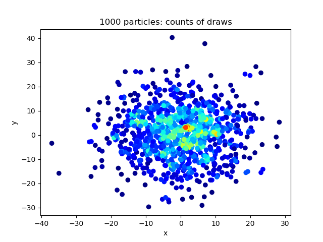
Python package to sample pairs of particles in n dims from discrete Gaussian distribution. Given a set of n particles with positions in d-dimensional space denoted by x_i for i=0,1,...,n. We want to sample a pair of particles i,j where i =/= j, where the probability for sampling this pair is given by p(i,j) ~ exp( - |x_i - x_j|^2 / 2 sigma^2 ) where we use |x| to denote the L_2 norm, and sigma is some chosen standard deviation.
lattgillespie
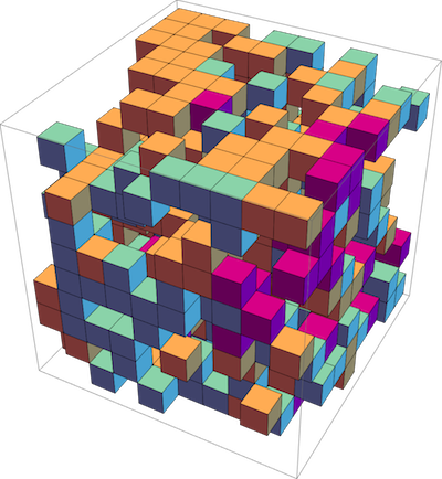
C++ library for Gillespie stochastic simulation algorithm on a lattice. Gillespie algorithm on a lattice in the single-occupancy regime, including diffusion (particles hopping between neighboring sites), unimolecular and bimolecular reactions. Supports 1D, 2D, 3D lattices.
Used in publication: Phys Rev E. 99, 063315 (2019)
Publication: Phys Rev E. 99, 063315 (2019)
C++ library for Gillespie stochastic simulation algorithm on a lattice. Gillespie algorithm on a lattice in the single-occupancy regime, including diffusion (particles hopping between neighboring sites), unimolecular and bimolecular reactions. Supports 1D, 2D, 3D lattices.
gillespie_simple
Python package for Gillespie stochastic simulation algorithm. Intended to be (1) easily understood, and (2) easily extended for your own projects.
L2ProjPathToGrid
C++ library for solving point to trajectory optimization problem. L2 project a path to a regular grid in arbitrary dimension, using cubic splines in the grid. Uses the popular Armadillo numerical library.
Apps
The Masked Manual (iOS)
The Masked Man iOS app - surgical mask and respirator data from the FDA and CDC

This app lets you search for surgical mask and respirator data. Currently this data is spread out across unstructured websites from the FDA and CDC/NIOSH and databases such as openFDA. The app uses webscraping and queries from these databases to bring mask qualifications to consumers. Computer vision lets users scan box packaging and easily find mask information.

Data visualizations
Convolution calculator for CNNs
Calculator for convolution layers in neural networks.
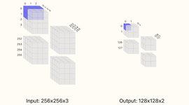
This calculator supports inputs which are 2-dimensional such as images or 1-dimensional such as timeseries (set one of the width/height dimensions to 1). You can visualize how the different choices tile your input data and what the output sizes will be. The basic formula for the number of outputs from the convolution operation is (W−F+2P)/S+1 where W is the size of the input (width or height), F is filter extent, P is the padding, and S is the stride. Note that for this calculator, only square filters are supported (the filter extent F controls both the width and height of the convolution) in reality, non-square convolutions are also possible.
Paper codes
2021
Physics-based machine learning for modeling stochastic IP3-dependent calcium dynamics
arXiv 2109.05053 (2021)
arXiv: arXiv:2109.05053
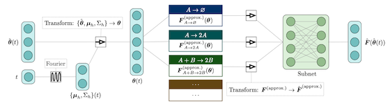
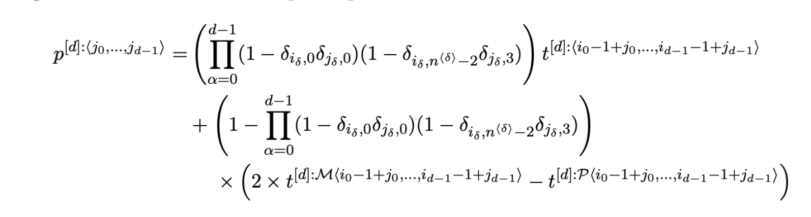
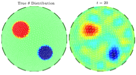
We present a machine learning method for model reduction which incorporates domain-specific physics through candidate functions. Our method estimates an effective probability distribution and differential equation model from stochastic simulations of a reaction network. The close connection between reduced and fine scale descriptions allows approximations derived from the master equation to be introduced into the learning problem. This representation is shown to improve generalization and allows a large reduction in network size for a classic model of inositol trisphosphate (IP3) dependent calcium oscillations in non-excitable cells.
2019
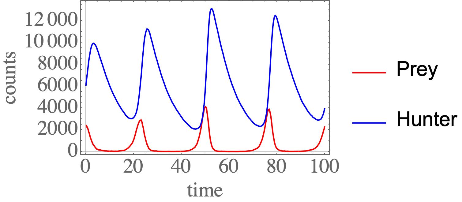
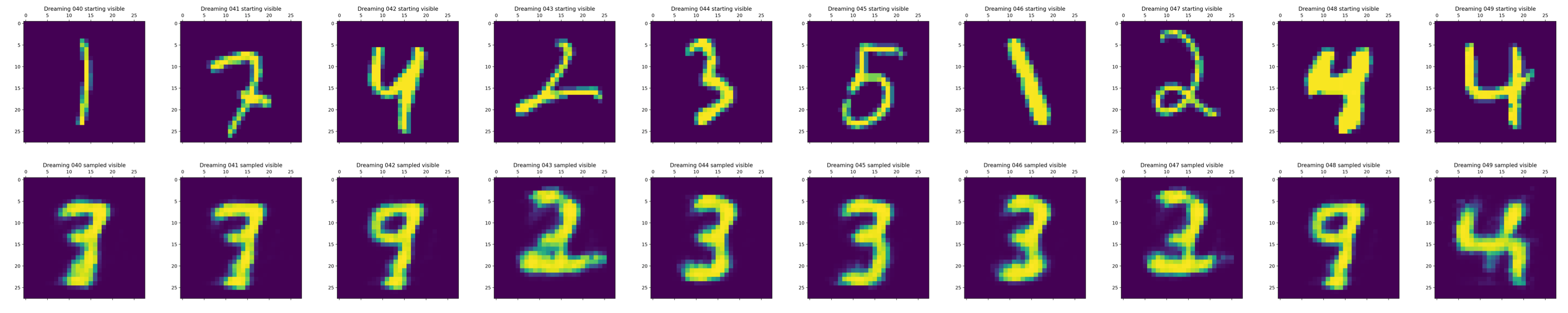
Deep Learning Moment Closure Approximations using Dynamic Boltzmann Distributions
arXiv 1905.12122 (2019)
arXiv: arXiv:1905.12122
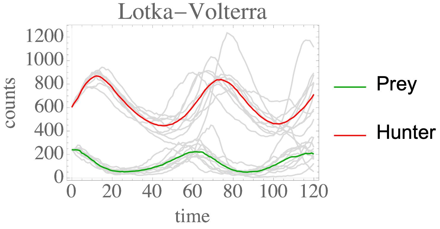
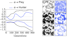
The moments of spatial probabilistic systems are often given by an infinite hierarchy of coupled differential equations. Moment closure methods are used to approximate a subset of low order moments by terminating the hierarchy at some order and replacing higher order terms with functions of lower order ones. For a given system, it is not known beforehand which closure approximation is optimal, i.e. which higher order terms are relevant in the current regime. Further, the generalization of such approximations is typically poor, as higher order corrections may become relevant over long timescales. We have developed a method to learn moment closure approximations directly from data using dynamic Boltzmann distributions (DBDs). The dynamics of the distribution are parameterized using basis functions from finite element methods, such that the approach can be applied without knowing the true dynamics of the system under consideration. We use the hierarchical architecture of deep Boltzmann machines (DBMs) with multinomial latent variables to learn closure approximations for progressively higher order spatial correlations. The learning algorithm uses a centering transformation, allowing the dynamic DBM to be trained without the need for pre-training. We demonstrate the method for a Lotka-Volterra system on a lattice, a typical example in spatial chemical reaction networks. The approach can be applied broadly to learn deep generative models in applications where infinite systems of differential equations arise.
2019
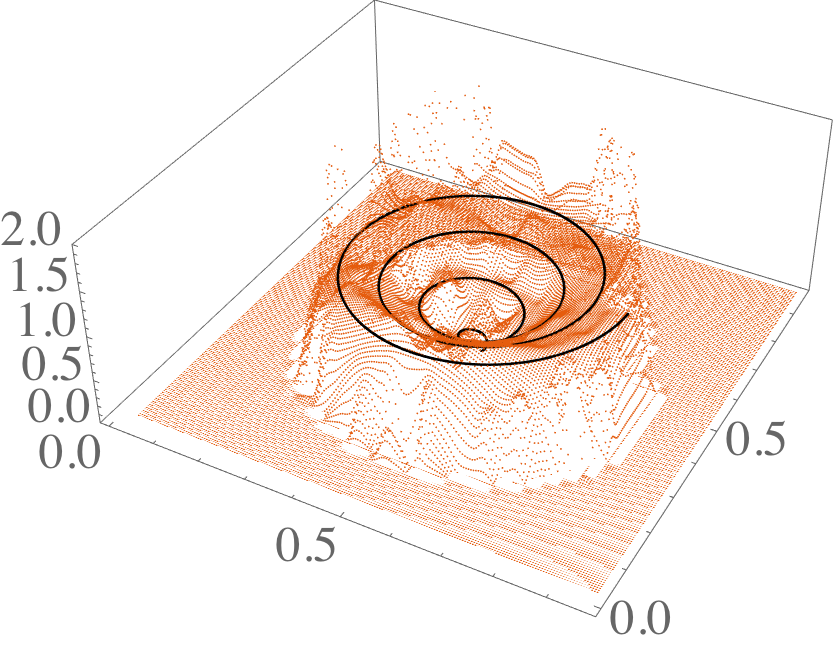
Learning moment closure in reaction-diffusion systems with spatial dynamic Boltzmann distributions
Phys Rev E. 99, 063315 (2019)
arXiv: arXiv:1808.08630
Publication: Phys Rev E. 99, 063315 (2019)
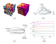
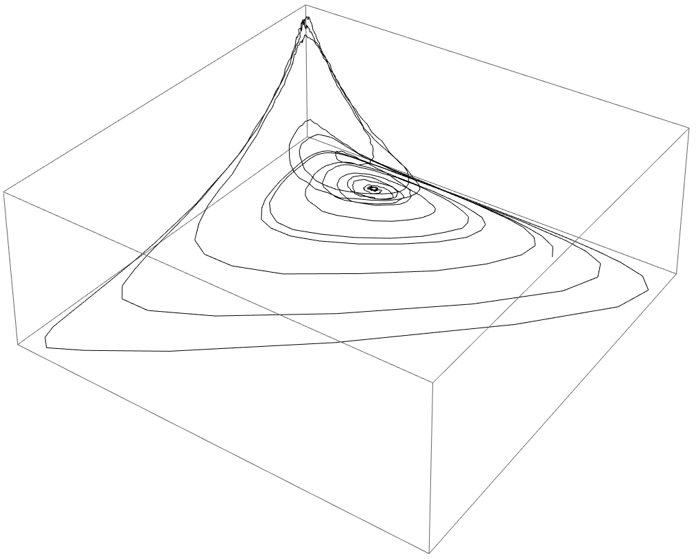
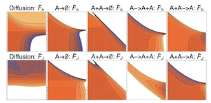
Many physical systems are described by probability distributions that evolve in both time and space. Modeling these systems is often challenging to due large state space and analytically intractable or computationally expensive dynamics. To address these problems, we study a machine learning approach to model reduction based on the Boltzmann machine. Given the form of the reduced model Boltzmann distribution, we introduce an autonomous differential equation system for the interactions appearing in the energy function. The reduced model can treat systems in continuous space (described by continuous random variables), for which we formulate a variational learning problem using the adjoint method for the right hand sides of the differential equations. This approach allows a physical model for the reduced system to be enforced by a suitable parameterization of the differential equations. In this work, the parameterization we employ uses the basis functions from finite element methods, which can be used to model any physical system. One application domain for such physics-informed learning algorithms is to modeling reaction-diffusion systems. We study a lattice version of the R{ö}ssler chaotic oscillator, which illustrates the accuracy of the moment closure approximation made by the method, and its dimensionality reduction power.
2018
Learning dynamic Boltzmann distributions as reduced models of spatial chemical kinetics
J. Chem. Phys 149 034107 (2018)
arXiv: arXiv:1803.01063
Publication: J. Chem. Phys 149 034107
Finding reduced models of spatially-distributed chemical reaction networks requires an estimation of which effective dynamics are relevant. We propose a machine learning approach to this coarse graining problem, where a maximum entropy approximation is constructed that evolves slowly in time. The dynamical model governing the approximation is expressed as a functional, allowing a general treatment of spatial interactions. In contrast to typical machine learning approaches which estimate the interaction parameters of a graphical model, we derive Boltzmann-machine like learning algorithms to estimate directly the functionals dictating the time evolution of these parameters. By incorporating analytic solutions from simple reaction motifs, an efficient simulation method is demonstrated for systems ranging from toy problems to basic biologically relevant networks. The broadly applicable nature of our approach to learning spatial dynamics suggests promising applications to multiscale methods for spatial networks, as well as to further problems in machine learning.
2014
Dynamic updating of numerical model discrepancy using sequential sampling
Inverse Problems 30 114019 (2014)
Publication: Inverse Problems 30 114019
This article addresses the problem of compensating for discretization errors in inverse problems based on partial differential equation models. Multidimensional inverse problems are by nature computationally intensive, and a key challenge in practical applications is to reduce the computing time. In particular, a reduction by coarse discretization of the forward model is commonly used. Coarse discretization, however, introduces a numerical model discrepancy, which may become the predominant part of the noise, particularly when the data is collected with high accuracy. In the Bayesian framework, the discretization error has been addressed by treating it as a random variable and using the prior density of the unknown to estimate off-line its probability density, which is then used to modify the likelihood. In this article, the problem is revisited in the context of an iterative scheme similar to Ensemble Kalman Filtering (EnKF), in which the modeling error statistics is updated sequentially based on the current ensemble estimate of the unknown quantity. Hence, the algorithm learns about the modeling error while concomitantly updating the information about the unknown, leading to a reduction of the posterior variance.
Tutorials
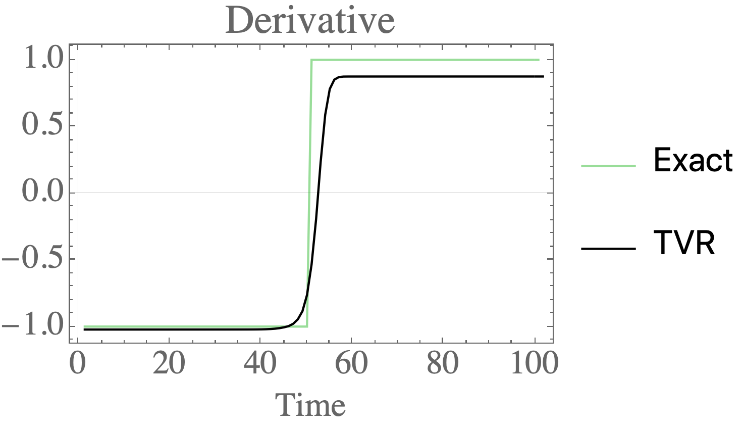
Total variation regularization for differentiation in Python
Differentiate noisy signals with total variation regularization in Python and Mathematica


Wolfram demonstrations
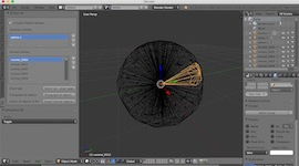
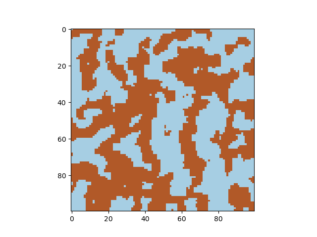
Cahn-Hilliard equation
The Cahn-Hilliard equation describes phase separation, for example of elements in an alloy. Starting from a random distribution of -1 and +1 (representing two species), the concentration evolves in time. Adjust the diffusion constant and the gamma parameter to obtain different solutions of the differential equations, and the timestep parameter to visualize the formation of domains.
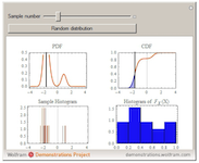
Visualizing the Probability Integral Transform
The probability integral transform is an important statement in statistics, used to generate random variables from a given continuous distribution by generating variables from the uniformly distribution on the interval [0,1]. Here, the principle is visualized by generating random variables from a given distribution, evaluating the CDF at these samples, and plotting the histogram of these values. With increasing samples, it is clear that this distribution is uniform on [0,1].
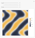
Pattern Formation in the Kuramoto Model
This demonstration shows artistic patterns that may arise in a two-dimensional Kuramoto model of coupled oscillators with variable phase shift. The oscillators are coupled to their nearest neighbors within an adjustable radius on a grid with periodic boundary conditions. The image shown displays the phase of each oscillator after evolving the system starting with random phases.
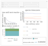
Gillespie Stochastic Simulation Algorithm
The Gillespie stochastic simulation algorithm is a Monte Carlo algorithm that simulates the time evolution of a chemical system according to its chemical master equation. In this demonstration, the reaction A+B\[LeftRightArrow]C is simulated with variable forward (Subscript[k, f]) and backward (Subscript[k, b]) rate constants and initial particle numbers. The demonstration shows the key steps of the Gillespie method. In the top left, the time until the next reaction is drawn from an exponential distribution. In the bottom left, the next reaction step (forward or backward) is randomly chosen based on the propensities of reaction. The plot on the right shows the timecourse of each species A,B,C. Use the "reaction event" slider to scroll through in time through the reactions that occur.
Electrodiffusion of Ions Across a Neural Cell Membrane
The Nernst-Planck equation describes the diffusion of ions in the presence of an electric field. Here, it is applied to describe the movement of ions across a neural cell membrane. The top half of the demonstration sets up the simulation, while the bottom displays the outcome. Four different ions that play key roles in neural dynamics - Na^+,\[CapitalKappa]^+,Ca^(2+),Cl^- - may be selected, and their interior and exterior concentrations adjusted using the sliders (shown in dotted and dashed green). The electric field across the membrane is assumed constant, such that the potential is linear, shown in the left plot. Three different initial concentration distributions are possible, shown by a dashed blue line in the right plot. The total simulation time may be set to either a relatively short or long time (slight delay to update). Once the parameters are set, press the "run simulation" button to generate the time course of the ion concentration, shown in solid blue. Move the simulation time slider to view the evolution of the distribution in time. If the parameters are changed, the curve turns to a dashed gray to indicate that the simulation should be run again. Equilibrium for the concentration of a single ion occurs when the potential is set to the Nernst reversal potential, and the initial distribution is set such that no ionic current exists, each shown in brown in the left and right plots.
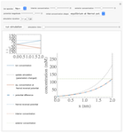
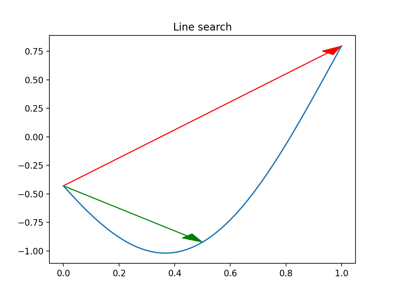
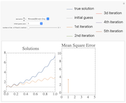
Approximating the Solution of Ordinary Differential Equations Using Picard's Method
An approximation to the solution to a first order ordinary differential equation is constructed using Picard's iterative method. The derivative function may be chosen using the drop down menu, as well as the initial guess in the algorithm. Increasing the number of iterations shown using the slider demonstrates the approach of the approximation to the true solution, shown in blue in the plot. The mean square error at each iteration is shown on the right.
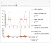
Sampling a Distribution using Slice Sampling
Slice sampling is a Markov chain Monte Carlo method used to sample points from a given distribution. The algorithm may be summarized as follows - given the previously sampled point, indicated by a purple dashed line, the corresponding ordinate is evaluated. A random number is drawn from a uniform distribution from zero to the ordinate value, indicated by a green circle. The intersections of a horizontal line (slice) at this value with the distribution curve is calculated. From the regions where the curve lies above the horizontal line, a second uniformly distributed random value is drawn, indicated by a red circle. This value is taken as the new sample point, and the algorithm repeats using this as the new starting point. A histogram of the sampled points is shown at the bottom. Adjust the slider to view the next or previous sample points. The distribution shapes may be chosen as Gaussian, gamma, or a linear combination of multiple Gaussian or gamma distributions. To generate new random variables for the current sample point, press the "generate random sample" button.
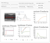
The Hodgkin-Huxley experiment
The Hodgkin-Huxley experiment measured the membrane conductances of sodium and potassium ions in the giant axon of the squid Loligo. This demonstration reproduces the essentails of the original experimental procedure.
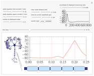
Action potential propagation along myelinated axons
An action potential travels down the myelinated axon of a neuron. In between myelin sheath sections (indicated by light blue boxes), at the nodes of Ranvier (indicated by vertical red lines in the plot), the potential is modeled by Hodgkin-Huxley dynamics. The propagation of the signal along the myelinated sections is described by the linear cable equation, whose space and time constants are variable, as well as the inter-node distance. The signal is initiated at the left end-node by an external current pulse or constant step of adjustable magnitude. The timecourse of a single point along the axon is displayed in the top-right. The speed of signal propagation can be visualized in real time using the autoplay feature of the time slider.
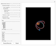
Object Tracking using the Kalman Filter
Track an object using the Kalman filter to reconstruct it's trajectory and velocity from noisy measurements in real time. The object, indicated by a blue pentagon, undergoes motion in a gravitional 1/r potential of adjustable magnitude created by an external mass, indicated by Mars, whose position can be controlled by the user in the pane on the right. The boundary conditions at the box edge are reflective. At regular intervals in time, measurements of the object's position are made with some additive measurement noise, drawn from a zero-mean Gaußian distribution. The Kalman filter is used to reconstruct both the trajectory of the object, shown in red, and the object's velocity, whose magnitude is indicated in the plot on the bottom left. The mean square error (MSE) between the reconstructed and true state vectors is shown as an estimate of the filter's performance in the middle left pane. The trace of the state covariance matrix is also shown in the middle right plane.
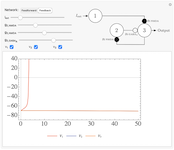
Feedforward and Feedback Inhibitory Neural Networks
Excitation and inhibition are two of the fundamental interactions between neurons. In neural networks, these processes allow for competition and learning, and lead to the diverse variety of output behaviors found in Biology. Two simple network control systems based on these interactions are the feedforward and feedback inhibitory networks. Feedforward inhibition limits activity at the output depending on the input activity. Feedback networks induce inhibition at the output as a result of activity at the ouput [1].
Other projects


Turing machines in Python
Undertand Turing machines with Python
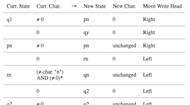
While you may not have access to a physical Turing machine, that should'nt stop you from simulating a Turing machine with… your computer! I will cover how Turing machines function, and Python code to build a simple one to test for alleged palindromes. I know that programs that check for palindromes are common exercise for programming beginners, and that you could simply check online or even copy some code in your favorite language. However, let's pretend that deep down you would really like to use a Turing machine for the task. This article is inspired by Chapter 5 of Perspectives in Computation by Robert Geroch - Amazon.