RBMs revisited in TensorFlow 2

Back to the bulk of the cake — unsupervised learning — with the latest tools.

Yann LeCunn stated at NIPS 2016:

If intelligence is a cake, the bulk of the cake is unsupervised learning, the icing on the cake is supervised learning, and the cherry on the cake is reinforcement learning (RL).

RBMs are at the heart of unsupervised learning — they’re about finding good latent representations of the data, which can then be used for some supervised task such as classification. They’re also more flexible than other generative frameworks — in contrast to VAEs, for example, the distribution over latent variables in RBMs is learned from data, rather than assumed Gaussian. Also, the learned energy function is a great framework on which to discuss “interpretability” in machine learning.

Last time RBMs were the talk of the town (mid-to-late 2000s), there wasn’t even TensorFlow v1. There are some implementations in that first TensorFlow v1 version floating out there — let’s revisit this important framework in TensorFlow 2.

The code for this project is on GitHub here.

Theory for gradients

Let’s briefly review the key theory for RBMs. A more detailed description can be found in this PDF in the GitHub repo.

An RBM only has one layer of visible units v and one layer of hidden units h. For this project we will only work with all-to-all connections in the RBM (every visible unit is connected to every hidden). There are no intra-layer connections (only inter-layer), which may appear in a general Boltzmann machine — hence the name restricted. For a lattice with visible units v and hidden units hwe wish to minimize the KL divergence:

where p is the true data distribution and \tilde{p} is the model distribution, given by:

where the partition function Z is:

A common form of the energy function is:

The gradients can be derived with the result (see the PDF in the GitHub repo for a detailed derivation):

where <...>_p is a moment under the data distribution, and <...>_\tilde{p} is a moment under the model distribution.

In practice, concerning the moments <...>, we usually cannot enumerate all possible states appearing in the sums. Therefore, these moments are estimated using batches. In the continuous case, let the batch be V_\tilde{p},H_\tilde{p},V_p,H_p of size N, typically small (N~5 or 10). For some observable:

such that the gradients are estimated as:

Theory for sampling

Where do such batches come from? They should be samples of the distributions p or \tilde{p} as appropriate.

Asleep phase

For sampling the model distribution \tilde{p} (aka ), we have several options:

• Without knowing further about \tilde{p}, we can always perform Markov Chain Monte Carlo (MCMC) to sample the distributions (other sampling methods be possible).
• For the particular energy function considered here, we can use , which works by iteratively sampling \tilde{p}(v_i | h) and \tilde{p}(h_i | v). These are given as follows:

Normally, you iteratively sample \tilde{p}(v_i | h) and \tilde{p}(h_i | v) for a long time to let the In , this procedure of iteratively sampling is performed only a few times (or even only once!), starting from an initial data vector v. This greatly improves computational efficiency.

After sampling, we obtain the desired samples for the batch V_{\tilde{p},i},H_{\tilde{p},i}. The sampling can be performed in for higher efficiency, evaluating all items in the batch V_\tilde{p},H_\tilde{p}.

In , we do not throw out the hidden states V_\tilde{p},H_\tilde{p} after one gradient step and restart from new data vectors v. Instead, we keep these states, and use them in the next gradient step again as the starting point for sampling \tilde{p}(v_i | h) and \tilde{p}(h_i | v) for a few more steps.

Awake phase

The samples V_p from the data distribution p (aka ) are obvious; they are provided as training data. The samples H_p are obtained by V_p and sampling \tilde{p}(h_i | v).

Implementation

It would be great if we could code up the KL divergence objective function onto a computer, but this is . Instead, we can make an important restriction:

Assume that our optimizer only uses first-order gradients.

If we make this restriction, we can consider the following objective function

which has the same first-order gradients as before. Note that the second-order gradients will obviously be incorrect!

This trick allows us to easily implement an RBM in TensorFlow, since we can now code up the objective function.

RBM class in TensorFlow 2

Let’s first code up the main RBM class. Some practical tricks can be found in Hinton’s guide here.

The complete class can be found in the GitHub repo here.

• The RBM class has a tf.Variable for the weights, visible bias and hidden bias.
• There are two further tf.Variable for the learning rates.
• We have already defined the optimizer as using Adam with the tf.keras.optimizers.Adam command, but it could also be e.g. SGD. The learning rates are passed as tf.Variable so we can change their value later.
• We have initialized some dummy structures to hold the chains for when we are using (perstistent CD).

Next, let’s define the loss function:

Again, an important note: this loss function reproduces the first order gradients, but not the second order gradients. But since we are using a first-order optimizer, this cheap trick will do. We also defined some helper methods to deal with dot products.

Next, the awake and asleep phases are performed as follows:

We haven’t yet defined the Gibbs sampler to do the actual sampling, but hopefully it is clear how the iterative sampling is performed. We are being careful to follow some obscured tricks on when to binarize the units (binary = True) vs. when to return raw probabilities.

Finally, let’s write the training loop:

• First we set the learning rates in case we are changing them between epochs, and reset the iteration count.
• We then loop over iterations in the while loop. Note that opt_weight.iterations is automatically updated when opt_weight.minimize is called.
• In each loop, we perform the awake and asleep phases of sampling.
• We then minimize the loss function with e.g.

self.opt\_weights.minimize(lambda: self.\_loss\_function(  
   =visible\_batch\_awake,  
   =hidden\_batch\_awake,  
   =self.visible\_batch\_asleep,  
   =self.hidden\_batch\_asleep),  
   =[  
      self.weights  
   ])

Note that the minimize function requires the loss function to be called without any arguments, hence the lambda . We also have two different optimizers for each the weights and the biases because it is common to use a smaller learning rate for the biases (0.1 or 0.01 times the learning rate for the weights).

If you got lost, the complete class can be found in the GitHub repo here.

Gibbs Sampler

The only missing part is the Gibbs sampler, coded in a GibbsSampler class. Since it isn’t the heart of this article, I’ll let you look at the code by yourself. The complete class can be found in the GitHub repo here.

Results

Let’s work with the old standard — MNIST. The training data looks as follows:

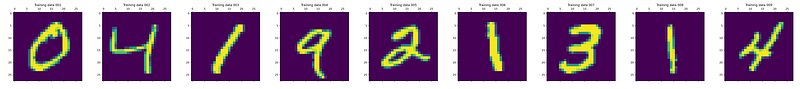
You can load and prepare the MNIST training data as follows:

Where we have flattened each image into a 1D vector, and normalized it into [0,1] . We have also chosen to have an equal number of visible and hidden units here — you can play around with this.

Let’s train the model with the following code:

We’re dividing the training into several epochs, and saving at each epoch with tf.train.CheckpointManager , since the training can take a while (on my computer ~15 minutes). You can list all the checkpoints that exist with manager.checkpoints , and restore a particular checkpoint with ckpt.restore(manager.checkpoints[i]) . Here we are only storing the weights and biases in the checkpoint, as defined in the tf.train.Checkpoint .

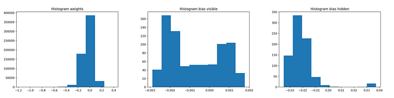
You can monitor convergence by observing the histograms of the learned weights and biases.

Let’s move on to the test data. We can “dream”, letting the RBM generate new digits starting from images in the testing set by CD sampling for many iterations as follows:

To invoke this dreaming routine, get the test data and feed some samples into the method:

The following shows examples of the dreamed digits. The top row shows the input digit; the bottom row shows the digit after CD sampling.

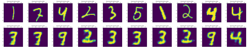
Some digits have switched, for example 4 into 9 and 5 into 3. Others have been maintained, such as 3 and the last 4. Others have been mutated into what almost looks like a digit, but not quite, such as 1 into something like a 3, or 2 into… also something like a 3!

Final thoughts

The complete code for this project is on GitHub here.

RBMs still have a lot of interest, particularly in scientific applications, for example in quantum physics and biophysics.

RBMs are closely related to deep Boltzmann machines (DBMs). Originally these were constructed by pre-training RBMs, which were then stacked. With a further centering trick, DBMs can be trained without pre-training.