Line search methods in optimization

And where are they in machine learning?

You can find the complete code for this tutorial on GitHub here.

We will review the theory for line search methods in optimization, and end with a practical implementation.

Motivation

In all optimization problems, we are ultimately interested in using a computer to find the parameters x that minimize some function f(x) (or -f(x) , if it is a maximization problem). Starting from an initial starting guess x_0, it is common to proceed in one of three ways:

• Gradient-free optimization— don’t laugh! Everyone does this. Here we are just guessing the next parameters:

for some random guess p to try to minimize the function, and evaluate the function f(x+p) at the new point to check if the step should be accepted. Actually we all do this — in almost any optimization algorithm, some hyperparameters need to be tuned (e.g. learning rates in machine learning, or initialization of parameters in any optimization problem). While some automatic strategies for tuning these also exist, it’s common to just try different values and see what works best.

• First order methods — these are methods that use the first derivative \nabla f(x) to evaluate the search direction. A common update rule is gradient descent:

for a hyperparameter \lambda .

• Second order methods —here we are using the Hessian \nabla^2 f(x) to pick the next step. A common update rule is Newton’s rule:

Often, a step size \eta \in (0,1] is included, which is sometimes known as the damped or relaxed Newton’s method.

This, however, is often not sufficient. First, the Hessian is usually expensive to compute. Second, we are generally interested in finding ai.e. one for which the product

is negative. This is equivalent to requiring that \nabla^2 f(x) is positive definite. To ensure that we are always following a descent direction, q replace the true inverse Hessian with a positive definite estimate, e.g. by regularizing it with a small diagonal matrix:

for a small \eps and I as the identity matrix. Note that we choose \eps = 0 if the true Hessian \nabla^2 f(x) is positive definite. Additionally, it is popular to construct an estimate from changing first order gradients that is also cheaper to compute, e.g. using the BFGS algorithm.

Any way that a new step is generated, in the end, we update the parameters as:

for some p . Note that since p is a descent direction, it always satisfies:

However, this step p is generated from only local information about the gradients — hence, it may be that the step ultimately does not minimize the function, i.e.

This is the opposite of what we want! We must come up with some other method to verify to adjust this step to ensure that we really are decreasing the function f — enter line search and trust region methods.

Line search methods vs Trust region methods

Line search methods start from the given direction p in which to go, and introduce a step length \alpha > 0to modulate how far along this direction we proceed. The line search problem is:

The specific condition can vary between line search methods — two common conditions are the Arimjo condition and the Wolfe condition, further discussed below. We can distinguish between two types of line searches:

• line search methods try to find \alpha > 0 such that f has really reached its minimum value over this interval.
• line search methods (more common) try to just ensure some sufficient condition that we have reduced the objective function.

Alternatively, trust-region methods can be used to accomplish the same goal. Here we do not start with a p from the zeroth/first/second order methods before. Instead, we start by constructing a model of the objective function at the current iteration using a Taylor series. A common choice is a second-order model:

Again, instead of using the real Hessian, it is common to use an approximation to it instead.

For small s , this will be a good approximation to f(x) by the definition of the Taylor series. For large s , it is a poor approximation. We therefore restrict our choice of s to lie within some trust region constraint:

For some radius r > 0 . We then try to pick the best s that minimizes our subject to this constraint:

After we have found this step, the objective function is reduced as:

Finally, we can modulate the trust region size r by considering how the actual decrease f(x) — f(x+s) compares to the predicted decrease from the model f(x) — m(s) . If they are similar, we can increase the trust region radius r. If the actual decrease is much smaller than the predicted decrease, then our model is bad and we should decrease the trust region radius r .

For further information, see e.g. the book “Trust-Region Methods” by Conn, Gould & Taint. Trust-region methods are very powerful! But line search methods are conceptually simple and work well in practice for integrating with existing optimizer implementations.

We next consider two popular line search conditions. A naive approach would just try to satisfy:

However, this does not prevent the step from . Enter the Armijo condition.

Armijo condition

The Armijo condition is a simple backtracking method that aims to satisfy:

where c \in (0,1) is a scaling factor, typically very small, e.g. c~1e-4 , and a(x) is the inner product of the gradient and descent direction defined above. Note that a(x) < 0 if p is a descent direction, which is always assumed to be the case here.

While the Armijo condition is not satisfied, we just backtrack starting from an initial step size \alpha_0 :

Where t \in (0,1) is a small parameter. t = 1/2 is a good starting point; closer to t = 1 the line search becomes more exact but slower; closer to t = 0 is faster but coarser.

Wolfe conditions

The Wolfe conditions are two conditions that must be satisfied:

1. The same Armijo condition as above:

1. An additional curvature condition:

where k \in (c,1) . This second condition ensures that the gradient in the objective function has by a sufficient amount — recall that a(x) < 0 for all descent directions, so it ensures that it is tending from negative to zero. This is important to ensure that the step length is not too small, i.e. we are not making progress toward the local minimum.

Implementation

The implementation of the Armijo backtracking line search is straightforward. Starting from a relatively large initial guess for the step size \alpha, just reduce it by a factor t \in (0,1) until it is satisfied.

The Wolfe conditions are more challenging because they require finding a step size that is sufficiently small to satisfy the Armijo condition, but also sufficiently large to satisfy the second Wolfe condition. Probably an existing implementation is better than any you would write yourself.

Let’s try an Armijo backtracking line search for the Newton method. First, the Newton method optimizer:

This is pretty simple:

• A run method that runs multiple optimization steps.
• A step method that runs every optimization step. Essentially, we evaluate the gradients:

gradients = self.gradient\_func(params)

and the regularized inverse Hessian (you must ensure that it is guaranteed positive definite such that it is a descent direction! See the main script below.):

rih = self.reg\_inv\_hessian(params)

Then form the update:

update = - np.dot(rih, gradients)

And run the line search:

alpha = self.run\_line\_search(update, params)  
update *= alpha

• The line search method run_line_search implements the backtracking, along with a helper method get_descent_inner_product that evaluates a(x) .

Next, let’s run it!

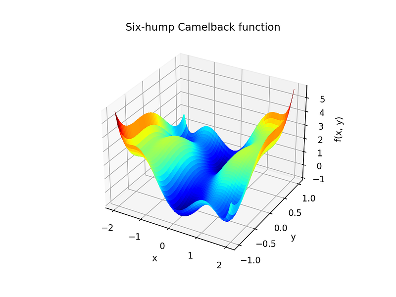
• We implemented the six-hump camelback objective function in obj_func :

• We implemented the gradient and the hessian , and the reg_inv_hessian :

This is obviously a pretty simple way to regularize it; we start with just a small diagonal matrix, and keep increasing the regularization parameter until the result is positive definite. I’m sure there are better methods (write me with suggestions!) — but this will do for now.

• Finally, we run the optimization routine:

params\_init = np.array([-1.1,-0.5])

converged, no\_opt\_steps, final\_update, traj, line\_search\_factors = opt.run(  
   =10,  
   =params\_init,  
   =1e-8,  
   =True  
)

The convergence is pretty quick — most initial points will take far fewer than 10 steps to converge.

The complete code is on GitHub here.

Results

Here is an example trajectory, starting from the cyan point to the red point:

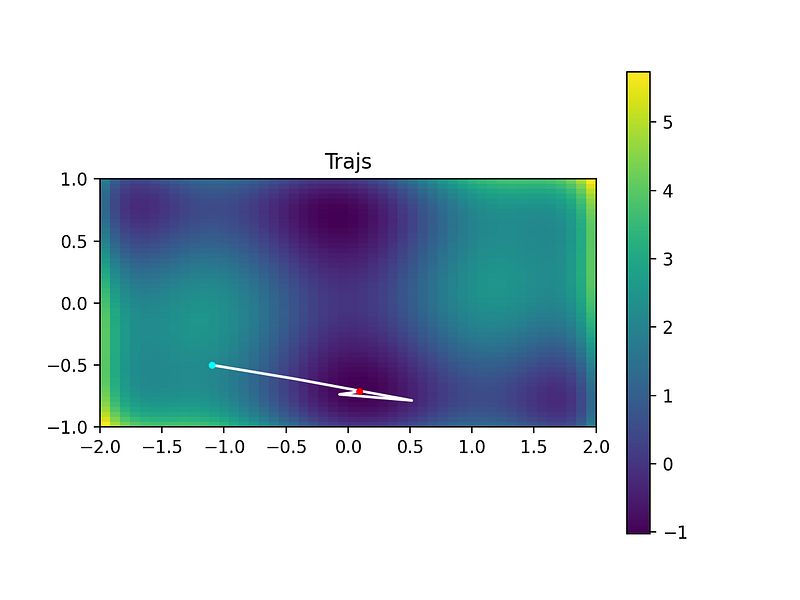
We can see it converges nicely to the global minimum in this case.

At step 3, a line search occurs:

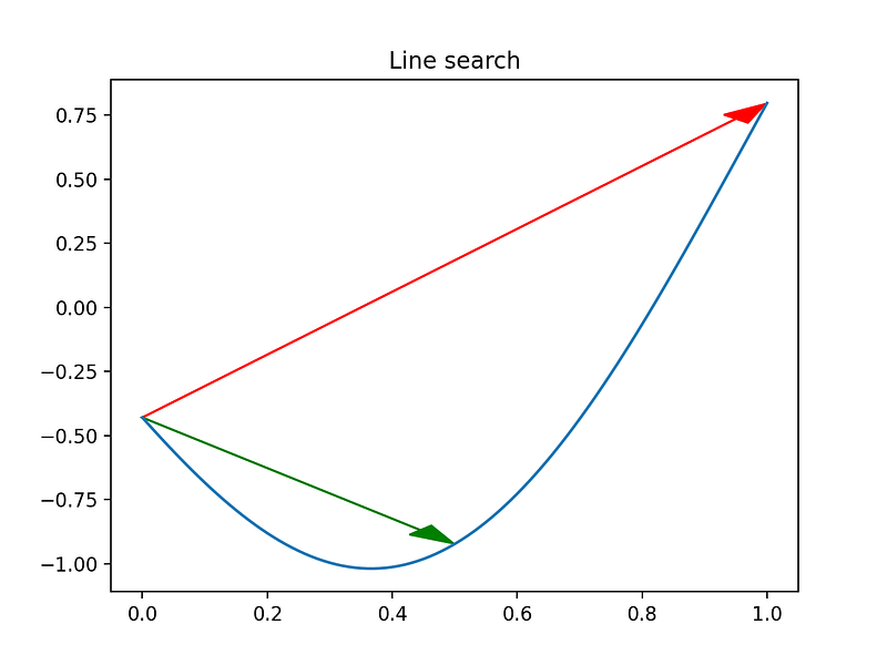
The blue line shows the objective function along the descent direction. The red arrow shows the initial proposed step (\alpha = 1 ). The green arrow shows the final step with \alpha = 0.5 — much better!

Final thoughts

In summary, the Armijo condition (first Wolfe condition) ensures in most cases that the step is not too large, i.e. jumping over the minimum. The second Wolfe condition guarantees that the step is not too small, i.e. that the increase in the gradient is sufficiently large.

Bonus: line search and trust region methods in machine learning

In machine learning settings, it is uncommon to find line search or trust region methods — or let’s call it: an open research direction. Machine learning methods rely on the idea of stochastic gradients — even though the objective function is defined over a large set of data, only a small batch is used to estimate the gradients. This noisy estimate is, well, noisy! But it’s also computationally much cheaper than evaluating the gradient over the full dataset — in fact, this is usually prohibitively expensive.

To perform the line search or trust region search, we would need to be able to evaluate the objective function at multiple points in parameter space at every optimization step. This, similarly, is too computationally expensive, but without further tricks, the estimate of the objective function from the small batch is too noisy to be used in a line search or trust region search.

The noisy gradients are also not purely a deficit. Machine learning usually involves optimization with many parameters, which introduces many unwanted local minima and saddle points. While it is generally accepted that no machine learning method converges to a global minimum, we still want to explore a large part of the parameter space to land somewhere beneficial to the task, rather than getting stuck in a local minimum. To do this, two tricks are beneficial:

1. Noisy gradients help us escape local minima.
2. Large learning rates can similarly help us break out if we are using first order methods like SGD or ADAM. This initially large learning rate is then usually reduced over training to improve convergence once we are in a “better” part of the parameter space.

The odd part is that line search methods can actually work against this in a sense. If we use enough data to get a good estimate of the objective function and then apply line search, it’s that we are no longer benefiting from the idea of taking a few noisy steps in a wrong direction with a large learning rate to avoid getting trapped. Even if we have enough computing power to estimate the objective function, this is a tricky balance to get right.