The simplest generative model you probably missed

A tutorial on probabilistic PCA.

There’s hardly a data scientist, scientist, programmer, or even marketing director who doesn’t about PCA (principal component analysis). It’s one of the most powerful tools for dimensionality reduction. If that marketing director is collecting survey data and looking to find target consumer groups for segmentation and analyzing the competition, PCA may very well be in play.

But you may have missed one of the simplest generative models that comes from an alternate view on PCA. If we derive PCA from a graphical model perspective, we arrive at probabilistic PCA. It allows us to:

• Draw new data samples (hence the generative label), and
• Generalize to Bayesian PCA where the dimensionality of the latent space can be estimated automatically (I’ll save this for a future article!), and
• Make a close connection between PCA and factor analysis (another article another day), and
• Formulate efficient expectation-maximization (EM) algorithms (another article…)…

and even neater applications! We’ll focus today on the first point and showing how it works, complemented with some Python (or Mathematica, if you like) code.

You can find the complete code on GitHub here.

---

Idea of probabilistic PCA

Let’s start out with the graphical model:

Pretty simple! Assume the latent distribution has the form:

The visibles are sampled from the conditional distribution:

Here W,\mu,\sigma^2 are the parameters to be determined from the dataset.

So everything’s a Gaussian! With this in mind, probabilistic PCA can be visualized best in the following stolen graphic from Bishop’s “Pattern Recognition and Machine Learning” text:

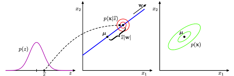
• : After sampling a variable from the latent distribution,
• : The visibles are drawn from an isotropic Gaussian (diagonal covariance matrix) around W * x_h + \mu .
• : The resulting marginal distribution for the observables is also a Gaussian, but not isotropic.

From the last two equations we can find the marginal distribution for the visibles is:

The parameters W,\mu,\sigma^2 can be determined by maximizing the log-likelihood:

where S is the covariance matrix of the data. The solution is obtained using the eigendecomposition of the data covariance matrix S:

Where the columns of U are the eigenvectors, and D is a diagonal matrix with the eigenvalues \lambda. Let the number of dimensions of the dataset be d (in this case, d=2). Let the number of latent variables be q, then the maximum likelihood solution is:

and \mu are just set to the mean of the data.

Here the eigenvalues \lambda are sorted from high to low, with \lambda_1 being the largest and \lambda_d the smallest. Here U_q is the matrix where columns are the corresponding eigenvectors of the q largest eigenvalues, and D_q is a diagonal matrix with the largest eigenvalues. R is an arbitrary rotation matrix — here we can simply take R=I for simplicity (see Bishop for a detailed discussion). We have discarded the dimensions beyond q — the ML variance \sigma^2 is then the average variance of these discarded dimensions.

You can find more information in the original paper: “Probabilistic principal component analysis” by Tipping & Bishop.

Let’s get into some code.

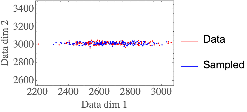
Load some data

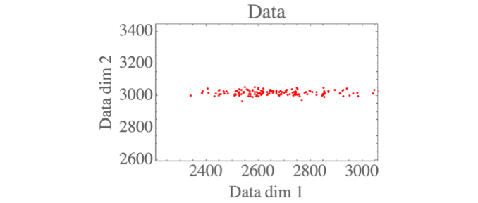
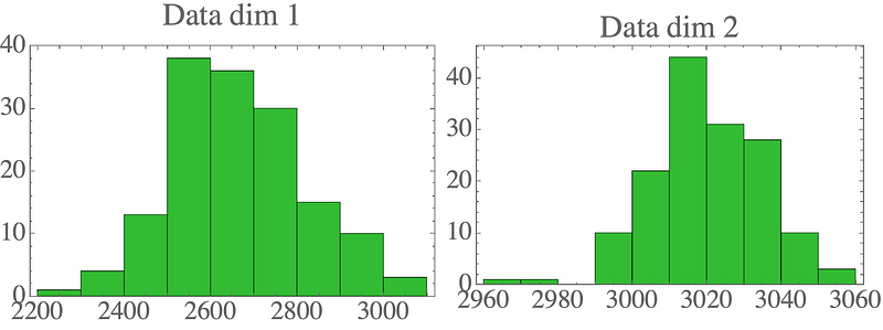
Let’s import and plot some 2D data:

where

loads a 2D text file.

You can see some plotting functions in use in the complete repo. Visualizing the data shows the 2D distribution:

Max-likelihood parameters

Here is the corresponding Python code to calculate these max-likelihood solutions:

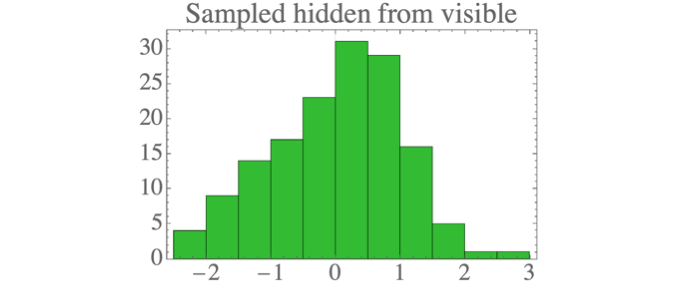
Sampling latent variables from the data

After determining the ML parameters, we can sample the hidden units from the visible according to:

You can implement it in Python as follows:

where we have defined:

The result is data which looks a lot like the standard normal distribution:

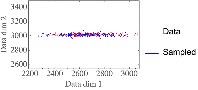
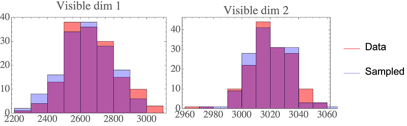
Generative mode: sample new data points

We can sample new data points by first drawing new samples from the hidden distribution (a standard normal):

and then sample new visible samples from those:

where we have defined:

The result are data points that closely resemble the data distribution:

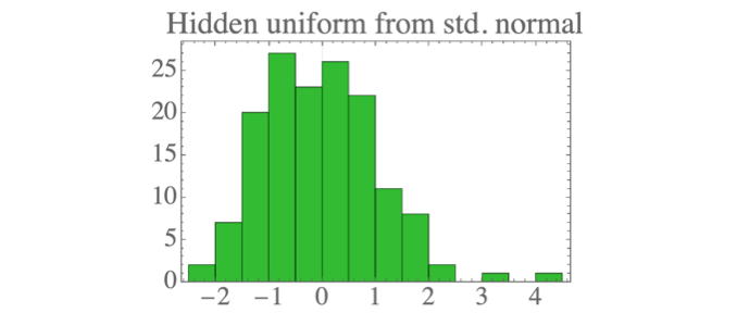
Rescaling the latent distribution

Finally, we can rescale the latent variables to have any Gaussian distribution:

For example:

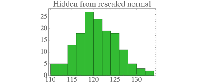
We can simply transform the parameters and then still sample new valid visible samples from those:

Nota that \sigma^2 is unchanged from before.

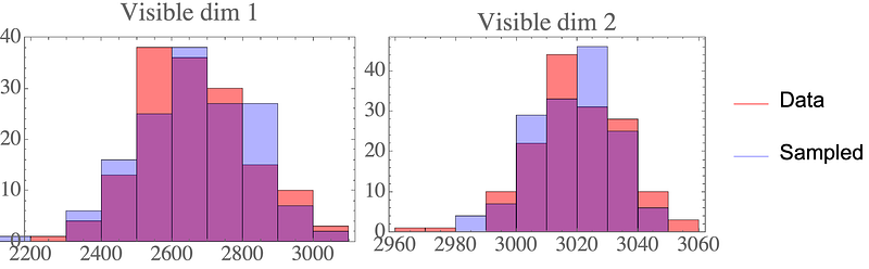
In Python we can do the rescaling:

and then repeat the sampling with the new weights & mean with the same function from before:

Again, the samples look like they could come from the original data distribution:

Final thoughts

We’ve shown how probabilistic PCA is derived from a graphical model. This Gaussian graphical model allows us a generative perspective on PCA, letting us draw new data samples. The latent distribution must be Gaussian, but can be any Gaussian — we can simply rescale the parameters. For non-Gaussian latent distributions, see e.g. independent component analysis (ICA).

In future articles, I’ll try to make the extension to Bayesian PCA, and the connection to factor analysis and general Gaussian graphical models.

You can find the complete code on GitHub here.