You’ve probably missed one of the greatest ML packages out there
And no, it’s not in Python. Or C++.
It might not even be in a language you already know, based on how relatively unpopular it is. But if you’ve studied math or physics at university you’ve probably at least heard of it.
I’m talking about Mathematica. And since version 11, it’s been possible to train neural networks directly in Mathematica.
Seriously? Mathematica?
Yes. Seriously. Keep reading.
If you’ve ever been interested in symbolic math, let’s get it out there: there’s really no parallel. Matlab just has basic symbolic capabilities, and is not really at all comparable (although both Mathematica and Matlab share the maddening indexing system that starts at one instead of zero…). Similarly, Python’s SymPy is a nice project, but it doesn’t at all parallel Mathematica’s capabilities. Mathematica can take integrals and derivatives, simplify complex expressions, and solve systems of equations analytically. Plus, Mathematica basically invented the idea of computational notebooks, rather than in Python, where Jupyter notebooks were really just an afterthought. The plots too look a lot nicer than those default matplotlib ones!
But what about symbolic math for ML? The answer should be obvious: automatic differentiation is much easier when you can do symbolic math.
If you’re coming from e.g. TensorFlow, you’ll be stunned how different the interface is for building neural networks. Mathematica focuses on building general graphs —but I think you’ll find it incredibly elegant!
In the rest of the article, I’m gonna show you the pieces to get started with ML in Mathematica.
Get Mathematica
Before you ask if it’s free — it is free-. Officially it’s proprietary and, of course, expensive — at the time of writing, a home desktop license runs $354. But there’s two large caveats here:
- If you’re a student or affiliated with a university, your institution probably provides it for free — this is probably the most common exposure to this great tool.
- If you’re not a university — Raspberry Pi OS (formerly Raspbian) ships with Mathematica for free. That means you can pick up a little $5 Raspberry Pi Zero (maybe even the ZeroW with built in WiFi!) and get a free working copy of Mathematica. From $354 down to $5 — how absurdly cool is that!

Three ways to make a neural network
- Load a pre-made one =
NetModel. - Make a simple layer-to-layer one, like the ones you might see in an introductory ML textbook =
NetChain. - Make a general graph =
NetGraph.
Let’s do each one in turn.
Load a pre-made network
The main command here is NetModel :
net = NetModel["LeNet Trained on MNIST Data"]
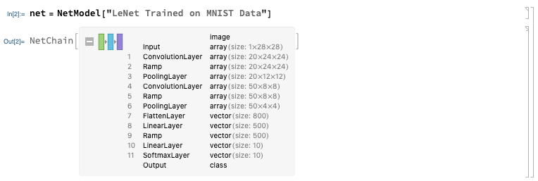
You can just fire up NetModel[] to see a list of all possible pre-loaded networks — I’ll put it at the bottom of this article.
Simple neural networks
A “simple” neural network in this case means a graph of layers where the i-th layer is connected to the i+1-st layer. This is done with the NetChain command:
net = NetChain[{
   LinearLayer[10],
   Tanh,
   LinearLayer[20],
   LogisticSigmoid
   },
  "Input" -> 10,
  "Output" -> 20
  ]
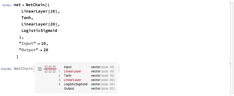
This introduced a couple new things:
- Layers: a
NetChainis composed of layers that are connected together. ALinearLayeris just one likeW * input + b. There’s lots more, likeElementwiseLayer,SoftmaxLayer,FunctionLayer,CompiledLayer,PlaceholderLayer,ThreadingLayer,RandomArrayLayer. Probably the most useful one isFunctionLayer, where you can apply a custom function (I’ll show you this layer). - Activation functions: you can stick in pretty much any function you like!
Tanh,Ramp(ReLU),ParametricRampLayer(leaky ReLU), andLogisticSigmoidare obvious choices, but you can use anything here. You can even repeat activation functions (for whatever reason) — no constraints here.
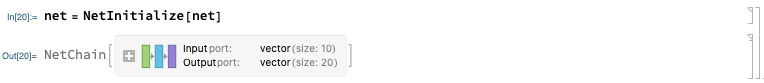
You can see the network is “uninitialized”. We can initialize the net with random weights and zero biases:
net = NetInitialize[net]
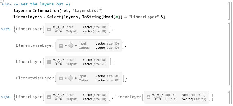
Let’s get those weights out. You can use Information[net, “Properties”] to query all the possible parameters. The layers can be extracted with:
layers = Information[net, "LayersList"]
linearLayers = Select[layers, ToString[Head[#]] == "LinearLayer" &]
The weights and biases can be obtained with:
weights1 = NetExtract[linearLayers[[1]], "Weights"]
Normal[weights1] // MatrixForm
biases1 = NetExtract[linearLayers[[1]], "Biases"]
Normal[biases1] // MatrixForm
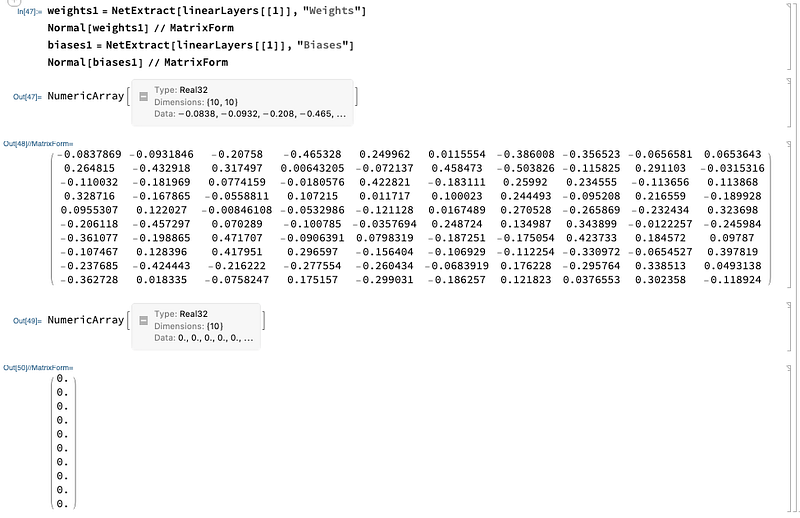
Note that Normal converts NumericalArray to the standard Mathematica list object that we can manipulate easily.
Make any arbitrary graph
Mathematica is great at graphs. The main command to make neural networks is NetGraph . This is where it gets really cool!
Let’s start with a network that takes a target vector of size 2 and another vector of size 2, and computes the L2 loss:
layerDefns = <|

   "l2" -> FunctionLayer[(#MyTarget - #MyLossInput)^2 &,
     "MyTarget" -> 2, "MyLossInput" -> 2, "Output" -> 2],
   "sum" -> SummationLayer[]
   |>;
layerConn = {{ NetPort["MyTarget"], NetPort["MyLossInput"]} ->
    "l2" -> "sum" -> NetPort["MyLoss"]};
l2lossNet = NetGraph[layerDefns, layerConn]
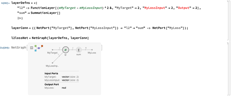
We see the format for NetGraph :
- An association (the Mathematica term for a dictionary of key/values) of name to layer.
- A list of layer names connected with arrows
->.
Also introduced is the notion of a NetPort . A NetPort is a named input/output of a network. You can clearly see the input ports on the left side of the layerConn definition, and the output ports on the right side:
layerConn = {{ NetPort["MyTarget"], NetPort["MyLossInput"]} ->
   "l2" -> "sum" -> NetPort["MyLoss"]};
The inputs are "MyTarget" and “MyLossInput” , and the output is “MyLoss" . You can clearly see these in the graph as well:
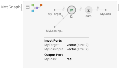
Look at this carefully — it shows you the dimensions of each connection in the graph, which is extremely helpful. The inputs are vectors of length 2, while the output is a scalar.
You can now reuse this graph in yet larger graphs, for example with another subnetwork:
subNet = NetChain[{LinearLayer[2], Tanh, LinearLayer[10], Tanh,
   LinearLayer[1]}]
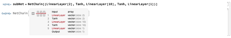
and the combination of the sub network and the loss network:
layerDefns = <|
   "sn1" -> subNet,
   "sn2" -> subNet,
   "l2loss" -> l2lossNet,
   "catentate" -> CatenateLayer[]
   |>;
layerConn = {
   NetPort["MyInput"] -> "sn1" -> "catentate",
   NetPort["MyInput"] -> "sn2" -> "catentate",
   {NetPort["MyTarget"], "catentate"} ->
    "l2loss" -> NetPort["MyLoss"]
   };
net = NetGraph[layerDefns, layerConn]
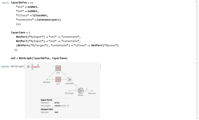
Let’s look at that more closely:
We have an input vector that get’s passed to in two separate channels of the subnetworks for a size of 2, then through different activation functions. These are then catenated (stacked), and passed into the loss function along with a target to finally obtain the loss.
Train networks
The command to train neural networks is NetTrain . Let’s train the net from the previous example. First, we need some data:
data = Flatten@Table[
    <|
     "MyInput" -> {x, y},
     "MyTarget" -> {Cos[x + y], Sin[x + y]}
     |>
    , {x, -1, 1, .02}
    , {y, -1, 1, .02}];
data[[1]]
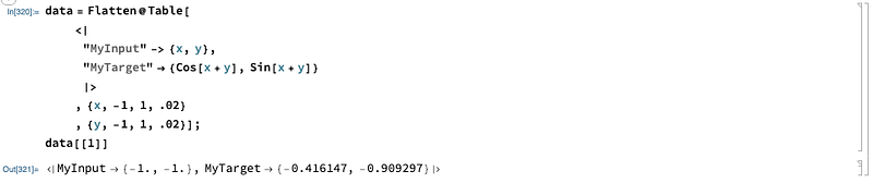
We can see each data sample is of the format of an association (dictionary) with every NetPort labeled.
Next the training:
trainedNet = NetTrain[net, data, LossFunction -> "MyLoss"]
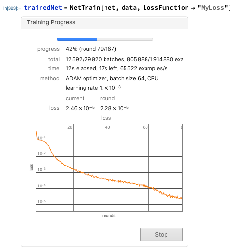
This is great — we get a simple overview and can visualize the training live. You can set different options — for example, the maximum number of iterations with:
NetTrain[..., MaxTrainingRounds->50000]
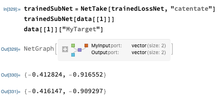
Finally, let’s evaluate the trained network. The network trainedNet outputs the full value of the loss function. Since we are interested more in the actual output, we can use NetTake to grab all layers up to and including the CatenateLayer :
trainedSubNet = NetTake[trainedNet, "catentate"]
trainedSubNet[data[[1]]]
data[[1]]["MyTarget"]
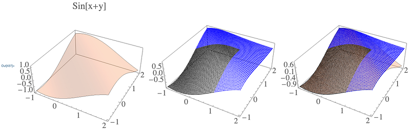
Let’s plot that and do some regression!
pts = Flatten[Table[
    {x, y, trainedSubNet[{x, y}][[2]]}
    , {x, -1, 2, .05}
    , {y, -1, 2, .05}], 1];
ptsTrain = Select[pts, #[[1]] <= 1 && #[[2]] <= 1 &];
ptsExtrapolate = Select[pts, #[[1]] > 1 || #[[2]] > 1 &];
pltPtsTrain = ListPointPlot3D[ptsTrain, PlotStyle -> Black];
pltPtsExtrapolate = ListPointPlot3D[ptsExtrapolate, PlotStyle -> Blue];
pltTrue =
  Plot3D[Sin[x + y], {x, -1, 2}, {y, -1, 2},
   PlotStyle -> Opacity[0.3], Mesh -> None, PlotLabel -> "Sin[x+y]",
   BaseStyle -> Directive[FontSize -> 24]];
Row[{
  pltTrue,
  Show[pltPtsTrain, pltPtsExtrapolate, PlotRange -> All],
  Show[pltPtsTrain, pltPtsExtrapolate, pltTrue, PlotRange -> All]
  }]
Final thoughts
You can read Mathematica’s more complete guide on neural networks here. However, it’s bit long…. If you prefer to just read through the API pages, here’s a better list from Wolfram.
I hope you got a sense of how powerful Mathematica’s neural networks are. The most powerful aspect is how you can build arbitrary graphs and loss functions — I don’t know any interface as capable as Mathematica’s for this, even if it is a bit different from TensorFlow. I really like the ability to combine networks easily with NetPorts and to visualize the dimensions of inputs and outputs easily. Additionally, the automatic monitoring training progress is incredibly useful.
Appendix: list of all possible pre-loaded networks at the time of writing
From the command NetModel[] :
2D Face Alignment Net Trained on 300W Large Pose Data
3D Face Alignment Net Trained on 300W Large Pose Data
AdaIN-Style Trained on MS-COCO and Painter by Numbers Data
Ademxapp Model A1 Trained on ADE20K Data
Ademxapp Model A1 Trained on Cityscapes Data
Ademxapp Model A1 Trained on PASCAL VOC2012 and MS-COCO Data
Ademxapp Model A Trained on ImageNet Competition Data
Age Estimation VGG-16 Trained on IMDB-WIKI and Looking at People Data
Age Estimation VGG-16 Trained on IMDB-WIKI Data
BERT Trained on BookCorpus and Wikipedia Data
BioBERT Trained on PubMed and PMC Data
BPEmb Subword Embeddings Trained on Wikipedia Data
CapsNet Trained on MNIST Data
Clinical Concept Embeddings Trained on Health Insurance Claims, Clinical Narratives from Stanford and PubMed Journal Articles
Colorful Image Colorization Trained on ImageNet Competition Data
ColorNet Image Colorization Trained on ImageNet Competition Data
ColorNet Image Colorization Trained on Places Data
ConceptNet Numberbatch Word Vectors V17.06
ConceptNet Numberbatch Word Vectors V17.06 (Raw Model)
CREPE Pitch Detection Net Trained on Monophonic Signal Data
CycleGAN Apple-to-Orange Translation Trained on ImageNet Competition Data
CycleGAN Horse-to-Zebra Translation Trained on ImageNet Competition Data
CycleGAN Monet-to-Photo Translation
CycleGAN Orange-to-Apple Translation Trained on ImageNet Competition Data
CycleGAN Photo-to-Cezanne Translation
CycleGAN Photo-to-Monet Translation
CycleGAN Photo-to-Van Gogh Translation
CycleGAN Summer-to-Winter Translation
CycleGAN Winter-to-Summer Translation
CycleGAN Zebra-to-Horse Translation Trained on ImageNet Competition Data
Deep Speech 2 Trained on Baidu English Data
Dilated ResNet-105 Trained on Cityscapes Data
Dilated ResNet-22 Trained on Cityscapes Data
Dilated ResNet-38 Trained on Cityscapes Data
DistilBERT Trained on BookCorpus and English Wikipedia Data
EfficientNet Trained on ImageNet
EfficientNet Trained on ImageNet with AutoAugment
EfficientNet Trained on ImageNet with NoisyStudent
ELMo Contextual Word Representations Trained on 1B Word Benchmark
Enhanced Super-Resolution GAN Trained on DIV2K, Flickr2K and OST Data
ForkNet Brain Segmentation Net Trained on NAMIC Data
Gender Prediction VGG-16 Trained on IMDB-WIKI Data
GloVe 100-Dimensional Word Vectors Trained on Tweets
GloVe 100-Dimensional Word Vectors Trained on Wikipedia and Gigaword 5 Data
GloVe 200-Dimensional Word Vectors Trained on Tweets
GloVe 25-Dimensional Word Vectors Trained on Tweets
GloVe 300-Dimensional Word Vectors Trained on Common Crawl 42B
GloVe 300-Dimensional Word Vectors Trained on Common Crawl 840B
GloVe 300-Dimensional Word Vectors Trained on Wikipedia and Gigaword 5 Data
GloVe 50-Dimensional Word Vectors Trained on Tweets
GloVe 50-Dimensional Word Vectors Trained on Wikipedia and Gigaword 5 Data
GPT2 Transformer Trained on WebText Data
GPT Transformer Trained on BookCorpus Data
Inception V1 Trained on Extended Salient Object Subitizing Data
Inception V1 Trained on ImageNet Competition Data
Inception V1 Trained on Places365 Data
Inception V3 Trained on ImageNet Competition Data
LeNet
LeNet Trained on MNIST Data
Micro Aerial Vehicle Trail Navigation Nets Trained on IDSIA Swiss Alps and PASCAL VOC Data
MobileNet V2 Trained on ImageNet Competition Data
Multi-scale Context Aggregation Net Trained on CamVid Data
Multi-scale Context Aggregation Net Trained on Cityscapes Data
Multi-scale Context Aggregation Net Trained on PASCAL VOC2012 Data
OpenFace Face Recognition Net Trained on CASIA-WebFace and FaceScrub Data
Pix2pix Photo-to-Street-Map Translation
Pix2pix Street-Map-to-Photo Translation
Pose-Aware Face Recognition in the Wild Nets Trained on CASIA WebFace Data
Pre-trained Distilled BERT Trained on BookCorpus and English Wikipedia Data
ResNet-101 for 3D Morphable Model Regression Trained on Casia WebFace Data
ResNet-101 Trained on Augmented CASIA-WebFace Data
ResNet-101 Trained on ImageNet Competition Data
ResNet-101 Trained on YFCC100m Geotagged Data
ResNet-152 Trained on ImageNet Competition Data
ResNet-50 Trained on ImageNet Competition Data
RetinaNet-101 Feature Pyramid Net Trained on MS-COCO Data
RoBERTa Trained on BookCorpus, English Wikipedia, CC-News, OpenWebText and Stories Datasets
SciBERT Trained on Semantic Scholar Data
Self-Normalizing Net for Numeric Data
Sentiment Language Model Trained on Amazon Product Review Data
Single-Image Depth Perception Net Trained on Depth in the Wild Data
Single-Image Depth Perception Net Trained on NYU Depth V2 and Depth in the Wild Data
Single-Image Depth Perception Net Trained on NYU Depth V2 Data
Sketch-RNN Trained on QuickDraw Data
Squeeze-and-Excitation Net Trained on ImageNet Competition Data
SqueezeNet V1.1 Trained on ImageNet Competition Data
SSD-MobileNet V2 Trained on MS-COCO Data
SSD-VGG-300 Trained on PASCAL VOC Data
SSD-VGG-512 Trained on MS-COCO Data
SSD-VGG-512 Trained on PASCAL VOC2007, PASCAL VOC2012 and MS-COCO Data
U-Net Trained on Glioblastoma-Astrocytoma U373 Cells on a Polyacrylamide Substrate Data
Unguided Volumetric Regression Net for 3D Face Reconstruction
Vanilla CNN for Facial Landmark Regression
Very Deep Net for Super-Resolution
VGG-16 Trained on ImageNet Competition Data
VGG-19 Trained on ImageNet Competition Data
VGGish Feature Extractor Trained on YouTube Data
Wide ResNet-50-2 Trained on ImageNet Competition Data
Wolfram AudioIdentify V1 Trained on AudioSet Data
Wolfram C Character-Level Language Model V1
Wolfram English Character-Level Language Model V1
Wolfram ImageIdentify Net V1
Wolfram JavaScript Character-Level Language Model V1
Wolfram LaTeX Character-Level Language Model V1
Wolfram Python Character-Level Language Model V1
Yahoo Open NSFW Model V1
YOLO V2 Trained on MS-COCO Data
YOLO V3 Trained on Open Images Data
Contents
Oliver K. Ernst
December 28, 2020