How to differentiate noisy signals

Without amplifying the noise!

Noise, noise everywhere. Image by alexey.shikov (License: CC0 1.0)

That’s the real trick — how to differentiate a noisy signal, without amplifying the noise. It comes up all the time:

You’re taking data from an infrared sensor or some other displacement sensor, and want to compute velocity and acceleration.
You’re tracking the price of your favorite stock, option, or GME short and think your prediction will give you the edge to make money (spoiler: it won’t…).

The well known problem for a noisy signal is that:

Differentiation amplifies noise.
Integration introduces drift.

If you think you’re clever, you’ll come up with some sort of smoothing approach to combat that. You’ll try a low-pass filter on the signal to eliminate the noise, and then you’ll differentiate it. Maybe you’ll even smooth that derivative again, and hope that the integrated signal will still be accurate! But no approach with smoothing will be without problems — the real secret is to regularize the differentiation itself.

I recently came across Total Variation Regularization (TVR)— you may have encountered this before in the field of image denoising, similar to the description you’ll find on Wikipedia. Here I’ll show you how it applies to differentiating noisy signals following this paper and this book (chapter 8). I’ll take you through the main idea and then on to some examples and code in Python and Mathematica.

You can find the complete code for this project on GitHub here.

Total-Variation Regularization (TVR)

Consider some vector of data f which contains the noisy data f_i for i=1,...,N-1 , so of length N. Here we consider the case where the data is evenly spaced with spacing \Delta x — “we leave the generalization to data with uneven spacing as an exercise to the reader” (have you ever read scarier words?). We’ll do everything in the discrete setting here; of course you can also more generally do it in continuous space.

Taking the derivative naively is given by:

There’s only N-1 of those. You can consider g_i as the derivative at the midpoint, i.e. if f_i corresponds to x_i , then g_i is the central difference, giving the derivative at 0.5*(x_i + x_{i+1}) . We can frame this as a matrix problem as well:

Here D is of size (N-1) x N. The anti-derivative operator is a bit harder to define:

The important part is the matrix A which implements the trapezoidal rule; the rest is for the initial point. Note that here A is of size (N-1) x (N-1) .

In total variation regularization, we instead frame the derivative as an optimization problem, with objective function S(u) for the desired derivative vector u of length N-2:

Let’s look at the first term:

\alpha is a tunable hyperparameter. A greater \alpha leads to a smoother derivative u ; a smaller \alpha will lead to a more faithful reproduction of the data.
D is a matrix that implements the differentiation operator — it’s up to you but let’s just use the one from before.
We are effectively regularizing the second derivative, which encourages the resulting derivative to not have discontinuous.

In the second term:

A is a matrix that implements the anti-differentiation operator. We’ll follow the example of using the trapezoidal rule (see code below), since it’s better than just the raw Euler formula above. We can discard the first point since it is given.
The L2 loss in the second term (the data fidelity term) is a good choice if you believe the noise in your data is Gaussian, which also works well in general — but this should be changed if you have a specific know noise distribution (see this paper).

As is usual for optimization problems, the optimizer method is critical. While you can try your luck with the usual gradient descent or Newton’s method, the winner appears to be lagged diffusivity fixed point iteration. All three are described in Chapter 8 of this book, so we’ll leave the description to that, and instead make plain the relevant equations to update from u_k to u_{k+1}:

This implementation writes out giant differentiation and integration matrices D,A . A more efficient version can be devised for large problems where writing out giant matrices is too expensive.

If you want your own implementation, you can use these equations. Else, you can find the Mathematica and Python implementations in this repo.

Simple example: an absolute value function

As a simple example, we’ll steal a pretty amazing one from following this paper. It’s an absolute value function that is significantly corrupted with Gaussian noise:

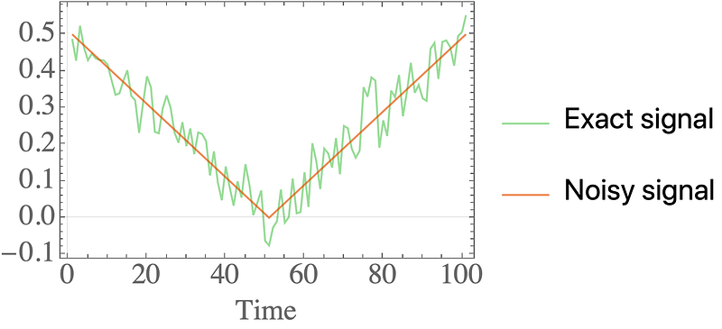
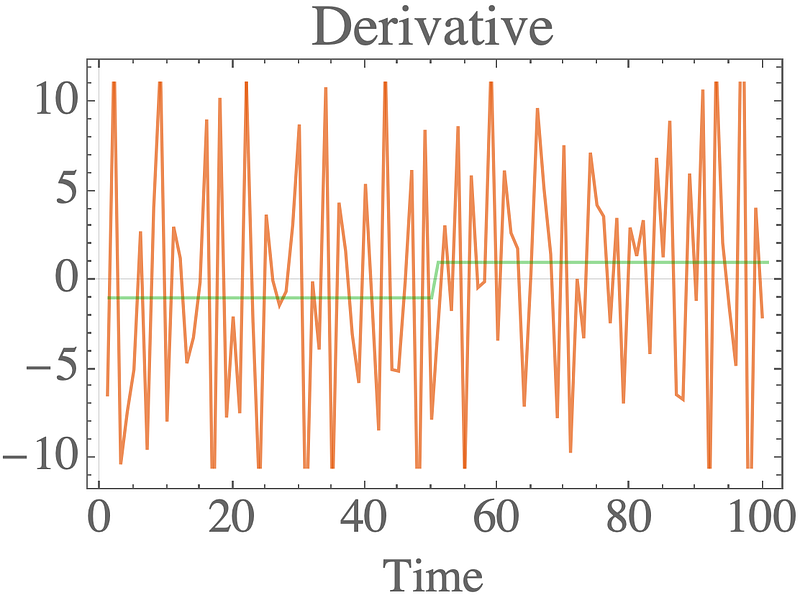
Taking the derivative should yield a step function (we’ll ignore the point at which it is undefined), but differentiating the noisy signal gives an incredibly unsatisfactory result.

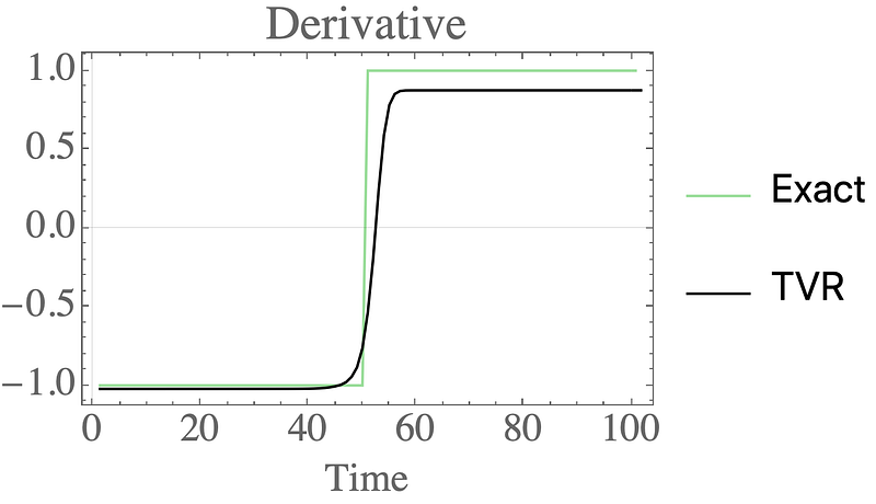
Applying TVR instead gives a stunningly good result — the derivative is sharp where it should be, and flat otherwise:

Detailed example: a damped oscillator

The previous example is eye-fetching, but it’s bit overly simple since the derivative only attains two values. As a more complete test we’ll consider a damped oscillator:

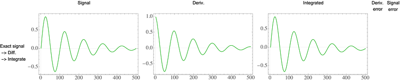
which again will be corrupted with Gaussian noise:

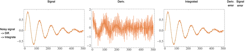
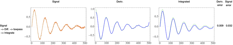
As before, the derivative is terribly corrupted by noise! Let’s try to come up with a homemade solution involving smoothing. Let’s try a low-pass filter on the signal before we differentiate:

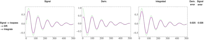
Now the derivative looks smoother, but (1) the initial points doesn’t look good, and (2) the integrated signal is off in the peaks. Maybe you believe the chosen cutoff is too low — let’s try again with a higher cutoff:

Now the integrated signal looks better, but the derivative looks too noisy! That’s the problem with these approaches — you end up balancing the smoothness of the derivatives and the accuracy of the integrated signal. And before you think a moving average will do better than a low-pass filter — forget it!

It actually feels like we’ve got the worst of both worlds — a noisy derivative and drift in the integration.

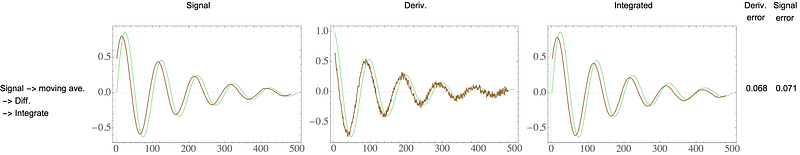
We can try two more strategies:

Taking the derivative of the raw noisy signal and then low-pass filtering the derivative:

The derivative looks better, but the integrated signal shows some drift from the true solution.

Low-pass everything: first low-pass the noisy signal, then differentiate, then low-pass the differentiated signal. This involves two rounds of hand-tuning filters, and the result is….

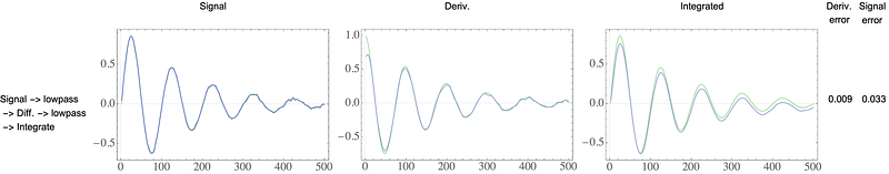
Still not good! Noisy in the end of the derivative, inaccurate in the beginning, and drift in the integration.

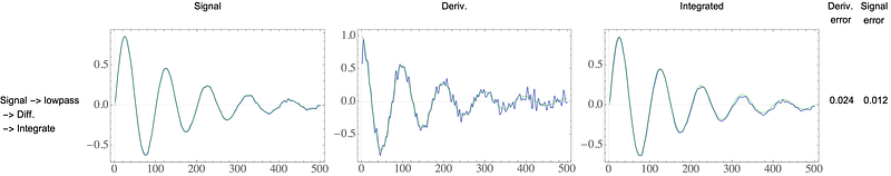
TVR again

Let’s look at how TVR does for this task.

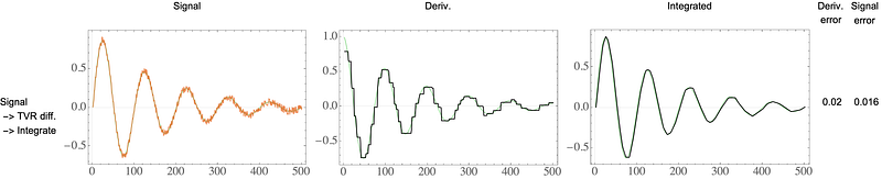
You may be disappointed — but wait.

Don’t judge too soon! The derivative looks a bit choppy — but the integrated signal looks amazing! No drift and smooth. This is by design of TVR — the optimization problem aims to minimize the error in integrated derivative. One strategy for making the derivative smoother is to increase \alpha in the optimization, but this sacrifices the accuracy of the integrated signal. The real magic kicks in with a round of low-pass filtering the TVR derivative:

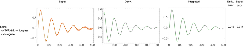
That’s a winner! A smooth & accurate derivative, and a smooth & accurate integrated signal, without drift.

Comparison together

You can compare all the approaches:

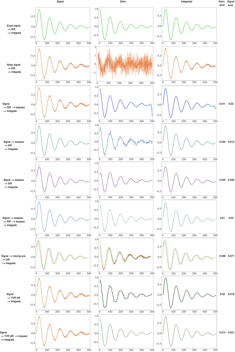
I’ve included estimates of the error in the derivative and the signal, which are computed from a vector x as:

Note that we divide by the range rather than the true signal, since this would amplify the error if the true signal is near zero.

In a single category (derivative or signal error), TVR does not have the lowest error; however it has low error across both categories. Additionally, it does not struggle with the initial points, which are very wrong for many of the approaches, and it does not introduce drift into the integration.

Final thoughts

The example for the absolute value function struck me how powerful this method is, and frankly, how underused it is. So stop rolling your own smoothing or averaging schemes and jump on the differentiation by total variation regularization wagon! It involves a little optimization, but the lagged diffusivity fixed point method gives quick convergence.

You can check out the code for this project on GitHub here.