Estimating constrained precision matrices with TensorFlow
Gaussian graphical models are defined by the structure of the precision matrix. From a fixed structure, how we estimate the values of the precision matrix? I will show you two slightly different problems using TensorFlow.

You can see the GitHub repo for this project here. The corresponding package can also be installed with
pip install tfConstrainedGauss
A detailed write up can also be found in the PDF in the [latex](https://github.com/smrfeld/tf-constrained-gauss/blob/main/latex/constrained_gauss.pdf) folder for this repo.
The problem we’re trying to solve
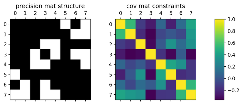
In a Gaussian graphical model, nodes denote random variables, and edges denote interactions. Which edges exist defines the structure of the precision matrix. For example, for the graphical model:
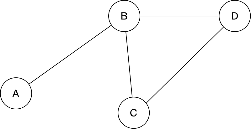
the structure of the precision matrix is:

From a given pile of data, we get a covariance matrix from which we would like to estimate the precision matrix. In some applications the goal is to also find the structure of the precision matrix — this is typically done with some form of lasso regularization to knock out small elements. In this article & corresponding Python package, we only consider the case where the structure of the precision matrix is known and fixed (but not its values).
The problem to estimate the precision matrix in this case is one of mixed constraints:
- Constraints on the precision matrix are those which set some elements to zero.
- Constraints on the covariance matrix are those given by the data.
This then cannot be solved just by taking a matrix inverse — the problem is best solved by optimization.
Two methods are presented and implemented in the Python package, which are actually solving two slightly different problems:
- A maximum entropy (MaxEnt) method. Gaussian distributions are MaxEnt distributions: the constraints are some specified covariances between random variables, and the Lagrange multipliers are the elements of the precision matrix (the edges in the graphical model). Therefore, in this problem setup, the constraints given in the covariance matrix are only those elements corresponding to the non-zero elements of the precision matrix.
- A method which minimizes the product of precision and covariance matrix, which should give the identity matrix. In this problem setup, the full covariance matrix is specified as a constraint. Because of this, the problem is over-constrained, and while we may find a “good” solution in the sense that the product of precision and covariance matrices is close to the identity, the elements of the covariance matrix found may not be close to the specified constraints.
Let’s dive deeper into each.
MaxEnt-based method
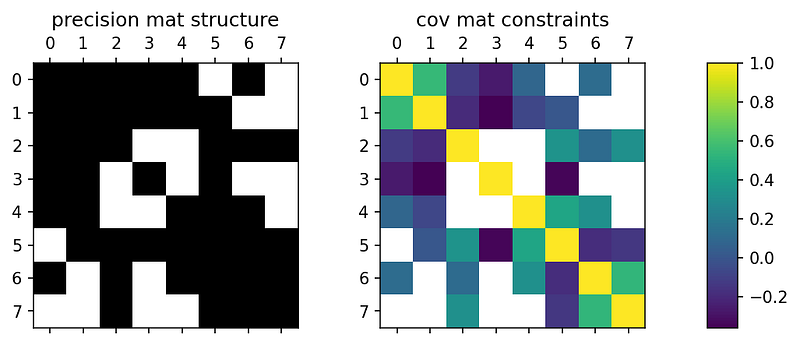
Given the structure of the n x n precision matrix (i.e. given the Gaussian graphical model), for example:

(note that the diagonal elements are always non-zero), and given the covariances for corresponding to every non-zero entry in P, i.e. in this example given the values:

the goal is to find the elements of P. In other words, every unique element (i,j) of the n x n symmetric matrix has a given constraint, either to a value in the covariance matrix, or a zero entry in the precision matrix.
This is a maximum entropy (MaxEnt) setup. The elements of the precision matrix pij are directly the interactions in the Gaussian graphical model; the moments they control in a MaxEnt sense are the covariances cij.
The problem can be solved in a number of ways, for example using Boltzmann machine learning, where we minimize:

where p(n) is the (unknown) data distribution that gave rise to the given covariances cij and q(n) is the Gaussian with precision matrix P. The gradients that result are the wake sleep phase:

In TensorFlow, we minimize the MSE loss for the individual terms, which results in the same first order gradients:

This minimization problem is implemented in the tfConstrainedGauss Python package. It uses Tensorflow to perform the minimization — see also the docs page.
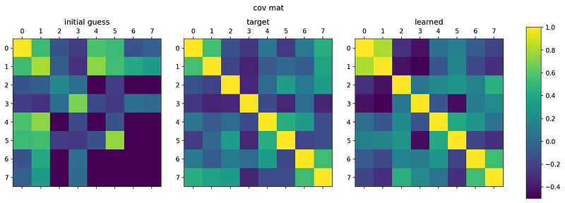
For the precision matrix structure and covariance matrix introduced previously, the result of solving the optimization problem is:
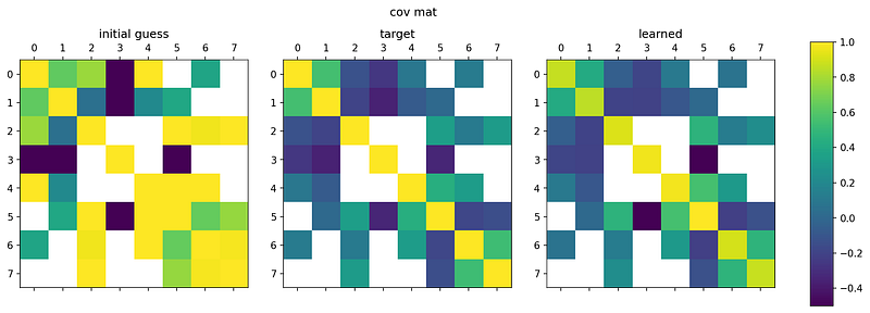
As we can see, the final learned covariance matrix closely matches the constraints.
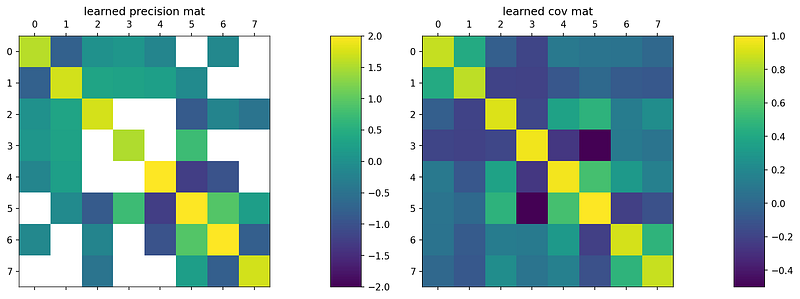
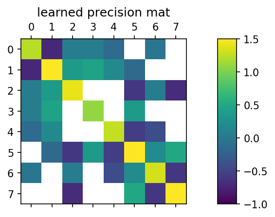
What is actually learned are the (non-zero) elements of the precision matrix:
The full covariance matrix on the right (the inverse of the precision matrix on the left) matches the constraints that are given, and fills in the remaining elements based on the specified graphical model.
Note that we can modify the learning algorithm slightly to learn each element of the covariance matrix with equal importance — we can use a weighted MSE loss:

where

A detailed write up can also be found in the PDF in the [latex](https://github.com/smrfeld/tf-constrained-gauss/blob/main/latex/constrained_gauss.pdf) folder for this repo.
Alternative: identity-based method
Given an n x n covariance matrix, here of size n=3:

and given the structure of the precision matrix (i.e. given the Gaussian graphical model), for example:

(note that the diagonal elements are always non-zero).
The goal is to find the elements of the precision matrix by:

where I is the identity.
Again, this is implemented in Tensorflow in the tfConstrainedGauss package.
The advantage of this approach is that it does not require calculating the inverse of any matrix, particularly important for large n.
The disadvantage of this approach is that the solution found for P may not yield a covariance matrix P^{-1} whose individual elements are close to those of C. That is, while P.C may be close to the identity, there are likely errors in every single element of P^{-1}.
This can be seen in the example from before:
Here the final learned covariance matrix on the right (the inverse of the learned precision matrix) actually does not really match the target covariance matrix (middle). The product of the learned precision matrix and given target covariance matrix may be close to the identity, but the inverse of that learned precision matrix — the learned covariance matrix — is off.
Incidentally, the learned precision matrix is:
Final thoughts
- Read more about this in PDF form here.
- Install the package using pip:
pip install tfConstrainedGauss
Contents
Oliver K. Ernst
October 2, 2021